Classical Mechanics Notes
Date: 2024/05/23Categories: Physics
Tags: Physics, Classical Mechanics
Read Time: 17 minutes
0.1 Contents
- 0.2 Kinematics
- 0.3 Forces
- 0.4 Work and Energy
- 0.5 Lagrangian Mechanics
- 0.5.1 Lagrangian
- 0.5.2 Euler-Lagrange Equation
- 0.5.3 Action Integral
- 0.5.4 Hamilton's Principle
- 0.5.5 Geodesic Equation
- 0.5.6 Generalised Coordinates in Lagrangian Mechanics
- 0.5.7 Example: Central Force
- 0.5.8 Lagrangian Mechanics with Constraints
- 0.5.9 System of Particles and Rigid Bodies
- 0.6 Small Oscillations
- 0.7 Normal Modes
- 0.8 Hamiltonian Mechanics
0.2 Kinematics
0.2.1 Newton's Second Law
Given a particle of mass %22%2F%3E%3C%2Fg%3E%3C%2Fg%3E%3Cdefs%3E%3Csymbol%20id%3D%22a%22%20overflow%3D%22visible%22%3E%3Cpath%20d%3D%22M9.855%206.63c-.915%200-1.71-.45-2.385-1.335-.135.885-.705%201.335-1.725%201.335-.885%200-1.65-.39-2.28-1.185-.12.66-.645%201.185-1.41%201.185-.615%200-1.065-.495-1.38-1.47-.165-.48-.24-.765-.24-.855%200-.135.075-.21.24-.21a.27.27%200%200%201%20.165.045c.075.135.12.24.15.345.27%201.14.615%201.71%201.02%201.71q.405%200%20.405-.63c0-.195-.075-.6-.24-1.215L1.32.945c-.06-.18-.135-.57-.135-.66%200-.3.165-.45.48-.45.3%200%20.51.15.615.45.015.075.12.45.285%201.095l.315%201.335.45%201.71c.165.345.42.69.75%201.05q.652.72%201.62.72c.495%200%20.735-.33.735-.975q0-.292-.225-1.215l-.405-1.71C5.7%201.86%205.46.96%205.34.48%205.325.375%205.31.315%205.31.285q0-.45.495-.45c.165%200%20.285.045.39.15.225.225.24.33.33.735l.885%203.555c.045.195.255.54.615%201.02.45.6%201.05.9%201.785.9.495%200%20.735-.33.735-.975%200-.585-.3-1.68-.915-3.285-.135-.345-.195-.63-.195-.825%200-.735.555-1.275%201.275-1.275.675%200%201.185.375%201.56%201.125.3.6.45%201.005.45%201.2%200%20.135-.075.21-.24.21-.105-.015-.21-.15-.285-.315C11.865.87%2011.385.27%2010.74.27c-.195%200-.3.15-.3.435%200%20.225.09.555.27%201.02.615%201.605.915%202.7.915%203.27%200%201.065-.705%201.635-1.77%201.635%22%2F%3E%3C%2Fsymbol%3E%3C%2Fdefs%3E%3C%2Fsvg%3E) and position vector
and position vector %22%2F%3E%3C%2Fg%3E%3C%2Fg%3E%3Cdefs%3E%3Csymbol%20id%3D%22a%22%20overflow%3D%22visible%22%3E%3Cpath%20d%3D%22M6.63%205.52c0%20.795-.81%201.23-1.59%201.23-1.05%200-1.65-.75-1.995-1.695V6.75l-2.49-.12v-.705c.93%200%201.035%200%201.035-.585V.705H.555V0l1.89.045c.57%200%201.53%200%202.07-.045v.705H3.21V3.33c0%201.05.375%202.88%201.875%202.88%200%200-.285-.255-.285-.69%200-.615.48-.915.915-.915s.915.315.915.915%22%2F%3E%3C%2Fsymbol%3E%3C%2Fdefs%3E%3C%2Fsvg%3E) ,
the second law states that the force
,
the second law states that the force %22%2F%3E%3C%2Fg%3E%3C%2Fg%3E%3Cdefs%3E%3Csymbol%20id%3D%22a%22%20overflow%3D%22visible%22%3E%3Cpath%20d%3D%22M10.125%206.585%209.66%2010.2H.585v-.705h1.62V.705H.585V0c.57.045%202.085.045%202.745.045.735%200%202.37%200%203.03-.045v.705H4.335v4.05h.75C6.525%204.755%206.66%204.11%206.66%203h.705v4.215H6.66c0-1.11-.12-1.755-1.575-1.755h-.75v4.035h2.1c2.415%200%202.76-1.155%202.985-2.91Z%22%2F%3E%3C%2Fsymbol%3E%3C%2Fdefs%3E%3C%2Fsvg%3E) acting on the particle
is equal to the time derivative of the momentum
acting on the particle
is equal to the time derivative of the momentum %22%2F%3E%3C%2Fg%3E%3C%2Fg%3E%3Cdefs%3E%3Csymbol%20id%3D%22a%22%20overflow%3D%22visible%22%3E%3Cpath%20d%3D%22M9%203.345C9%205.34%207.635%206.75%205.475%206.75c-1.125%200-1.92-.465-2.265-.735v.735L.555%206.63v-.705c.93%200%201.035%200%201.035-.57v-7.56H.555v-.705l1.89.045%201.89-.045v.705H3.3v2.79A2.92%202.92%200%200%201%205.22-.09C7.47-.09%209%201.26%209%203.345m-1.92%200C7.08%201.23%206.03.45%205.055.45c-.21%200-.915%200-1.59.81-.165.195-.165.21-.165.495v3.18c0%20.285.015.3.225.51.6.615%201.38.705%201.71.705%201.005%200%201.845-.915%201.845-2.805%22%2F%3E%3C%2Fsymbol%3E%3C%2Fdefs%3E%3C%2Fsvg%3E) of the particle:
of the particle:
%22%2F%3E%3Cuse%20xlink%3Ahref%3D%22%23b%22%20class%3D%22typst-text%22%20transform%3D%22matrix(1%200%200%20-1%2025.027%2030.565)%22%2F%3E%3Cuse%20xlink%3Ahref%3D%22%23c%22%20class%3D%22typst-text%22%20transform%3D%22matrix(1%200%200%20-1%2042.363%2020.41)%22%2F%3E%3Cuse%20xlink%3Ahref%3D%22%23d%22%20class%3D%22typst-text%22%20transform%3D%22matrix(1%200%200%20-1%2050.523%2020.41)%22%2F%3E%3Cuse%20xlink%3Ahref%3D%22%23c%22%20class%3D%22typst-text%22%20transform%3D%22matrix(1%200%200%20-1%2044.448%2040.855)%22%2F%3E%3Cuse%20xlink%3Ahref%3D%22%23e%22%20class%3D%22typst-text%22%20transform%3D%22matrix(1%200%200%20-1%2052.608%2040.855)%22%2F%3E%3Cpath%20fill%3D%22none%22%20stroke%3D%22%23000%22%20stroke-width%3D%22.72%22%20d%3D%22M42.363%2026.815h17.745%22%20class%3D%22typst-shape%22%2F%3E%3C%2Fg%3E%3C%2Fg%3E%3Cdefs%3E%3Csymbol%20id%3D%22a%22%20overflow%3D%22visible%22%3E%3Cpath%20d%3D%22M10.125%206.585%209.66%2010.2H.585v-.705h1.62V.705H.585V0c.57.045%202.085.045%202.745.045.735%200%202.37%200%203.03-.045v.705H4.335v4.05h.75C6.525%204.755%206.66%204.11%206.66%203h.705v4.215H6.66c0-1.11-.12-1.755-1.575-1.755h-.75v4.035h2.1c2.415%200%202.76-1.155%202.985-2.91Z%22%2F%3E%3C%2Fsymbol%3E%3Csymbol%20id%3D%22b%22%20overflow%3D%22visible%22%3E%3Cpath%20d%3D%22M10.47%205.505H1.2c-.24%200-.36-.12-.36-.345s.12-.345.36-.345h9.27c.24%200%20.36.12.36.345%200%20.18-.165.345-.36.345m0-2.82H1.2c-.24%200-.36-.12-.36-.345s.12-.345.36-.345h9.27c.24%200%20.36.12.36.345a.35.35%200%200%201-.36.345%22%2F%3E%3C%2Fsymbol%3E%3Csymbol%20id%3D%22c%22%20overflow%3D%22visible%22%3E%3Cpath%20d%3D%22M6.435%209.48%205.55%205.835c-.315.555-.75.84-1.335.84-.975%200-1.83-.495-2.58-1.5C.945%204.245.6%203.27.6%202.265c0-1.32.765-2.43%202.025-2.43C3.27-.165%203.9.18%204.5.885c.165-.57.675-1.05%201.38-1.05%201.035%200%201.365%201.23%201.59%202.34%200%20.135-.075.21-.225.21q-.202%200-.27-.315C6.675.885%206.315.285%205.91.285c-.255%200-.39.21-.39.615%200%20.225.03.465.09.705l2.13%208.58v.06a.26.26%200%200%201-.255.165c-.345%200-.975-.06-1.875-.165-.165-.015-.255-.135-.255-.345q0-.225.405-.225c.285%200%20.675.015.675-.195m-1.32-3.84c.15-.315.225-.525.225-.66a2%202%200%200%201-.045-.24L4.56%201.83a1.7%201.7%200%200%200-.285-.525C3.72.63%203.18.285%202.655.285c-.585%200-.885.45-.885%201.335q0%20.54.27%201.62c.315%201.275.765%202.145%201.32%202.61.3.255.585.375.87.375.405%200%20.705-.195.885-.585%22%2F%3E%3C%2Fsymbol%3E%3Csymbol%20id%3D%22d%22%20overflow%3D%22visible%22%3E%3Cpath%20d%3D%22M9%203.345C9%205.34%207.635%206.75%205.475%206.75c-1.125%200-1.92-.465-2.265-.735v.735L.555%206.63v-.705c.93%200%201.035%200%201.035-.57v-7.56H.555v-.705l1.89.045%201.89-.045v.705H3.3v2.79A2.92%202.92%200%200%201%205.22-.09C7.47-.09%209%201.26%209%203.345m-1.92%200C7.08%201.23%206.03.45%205.055.45c-.21%200-.915%200-1.59.81-.165.195-.165.21-.165.495v3.18c0%20.285.015.3.225.51.6.615%201.38.705%201.71.705%201.005%200%201.845-.915%201.845-2.805%22%2F%3E%3C%2Fsymbol%3E%3Csymbol%20id%3D%22e%22%20overflow%3D%22visible%22%3E%3Cpath%20d%3D%22M4.95%206.285c0%20.135-.15.21-.465.21H3.27q.585%202.34.585%202.43c0%20.315-.165.465-.48.465-.345%200-.555-.195-.645-.585l-.555-2.31H.84c-.33%200-.495-.015-.495-.33%200-.165.15-.24.465-.24h1.215C1.29%203%20.93%201.455.93%201.26c0-.84.57-1.425%201.41-1.425.57%200%201.065.255%201.5.78.36.435.615.855.78%201.26.06.165.09.255.09.3%200%20.135-.075.21-.225.21-.12%200-.21-.075-.27-.24C3.705.9%203.09.285%202.355.285c-.255%200-.39.21-.39.615%200%20.225.03.465.09.705l1.065%204.32h1.335c.39%200%20.495.03.495.36%22%2F%3E%3C%2Fsymbol%3E%3C%2Fdefs%3E%3C%2Fsvg%3E)
If the mass of the particle is constant, then the second law can be written
in terms of the acceleration %22%2F%3E%3C%2Fg%3E%3C%2Fg%3E%3Cdefs%3E%3Csymbol%20id%3D%22a%22%20overflow%3D%22visible%22%3E%3Cpath%20d%3D%22M8.295.36c0%20.345-.195.345-.39.345-.915.015-.915.21-.915.555v3.225c0%201.335-1.065%202.31-3.3%202.31-.855%200-2.685-.06-2.685-1.38%200-.66.525-.945.93-.945.465%200%20.945.315.945.945%200%20.45-.285.705-.33.735.42.09.9.105%201.08.105%201.125%200%201.65-.63%201.65-1.77v-.51C4.215%203.93.405%203.795.405%201.62.405.18%202.265-.09%203.3-.09c1.2%200%201.905.615%202.235%201.245C5.535.69%205.535%200%207.095%200h.72c.3%200%20.48%200%20.48.36M5.28%202.085C5.28.645%203.9.45%203.525.45%202.76.45%202.16.975%202.16%201.635c0%201.62%202.37%201.83%203.12%201.875Z%22%2F%3E%3C%2Fsymbol%3E%3C%2Fdefs%3E%3C%2Fsvg%3E) of the particle:
of the particle:
%22%2F%3E%3Cuse%20xlink%3Ahref%3D%22%23b%22%20class%3D%22typst-text%22%20transform%3D%22matrix(1%200%200%20-1%2025.027%2020.2)%22%2F%3E%3Cuse%20xlink%3Ahref%3D%22%23c%22%20class%3D%22typst-text%22%20transform%3D%22matrix(1%200%200%20-1%2040.863%2020.2)%22%2F%3E%3Cuse%20xlink%3Ahref%3D%22%23d%22%20class%3D%22typst-text%22%20transform%3D%22matrix(1%200%200%20-1%2054.033%2020.2)%22%2F%3E%3C%2Fg%3E%3C%2Fg%3E%3Cdefs%3E%3Csymbol%20id%3D%22a%22%20overflow%3D%22visible%22%3E%3Cpath%20d%3D%22M10.125%206.585%209.66%2010.2H.585v-.705h1.62V.705H.585V0c.57.045%202.085.045%202.745.045.735%200%202.37%200%203.03-.045v.705H4.335v4.05h.75C6.525%204.755%206.66%204.11%206.66%203h.705v4.215H6.66c0-1.11-.12-1.755-1.575-1.755h-.75v4.035h2.1c2.415%200%202.76-1.155%202.985-2.91Z%22%2F%3E%3C%2Fsymbol%3E%3Csymbol%20id%3D%22b%22%20overflow%3D%22visible%22%3E%3Cpath%20d%3D%22M10.47%205.505H1.2c-.24%200-.36-.12-.36-.345s.12-.345.36-.345h9.27c.24%200%20.36.12.36.345%200%20.18-.165.345-.36.345m0-2.82H1.2c-.24%200-.36-.12-.36-.345s.12-.345.36-.345h9.27c.24%200%20.36.12.36.345a.35.35%200%200%201-.36.345%22%2F%3E%3C%2Fsymbol%3E%3Csymbol%20id%3D%22c%22%20overflow%3D%22visible%22%3E%3Cpath%20d%3D%22M9.855%206.63c-.915%200-1.71-.45-2.385-1.335-.135.885-.705%201.335-1.725%201.335-.885%200-1.65-.39-2.28-1.185-.12.66-.645%201.185-1.41%201.185-.615%200-1.065-.495-1.38-1.47-.165-.48-.24-.765-.24-.855%200-.135.075-.21.24-.21a.27.27%200%200%201%20.165.045c.075.135.12.24.15.345.27%201.14.615%201.71%201.02%201.71q.405%200%20.405-.63c0-.195-.075-.6-.24-1.215L1.32.945c-.06-.18-.135-.57-.135-.66%200-.3.165-.45.48-.45.3%200%20.51.15.615.45.015.075.12.45.285%201.095l.315%201.335.45%201.71c.165.345.42.69.75%201.05q.652.72%201.62.72c.495%200%20.735-.33.735-.975q0-.292-.225-1.215l-.405-1.71C5.7%201.86%205.46.96%205.34.48%205.325.375%205.31.315%205.31.285q0-.45.495-.45c.165%200%20.285.045.39.15.225.225.24.33.33.735l.885%203.555c.045.195.255.54.615%201.02.45.6%201.05.9%201.785.9.495%200%20.735-.33.735-.975%200-.585-.3-1.68-.915-3.285-.135-.345-.195-.63-.195-.825%200-.735.555-1.275%201.275-1.275.675%200%201.185.375%201.56%201.125.3.6.45%201.005.45%201.2%200%20.135-.075.21-.24.21-.105-.015-.21-.15-.285-.315C11.865.87%2011.385.27%2010.74.27c-.195%200-.3.15-.3.435%200%20.225.09.555.27%201.02.615%201.605.915%202.7.915%203.27%200%201.065-.705%201.635-1.77%201.635%22%2F%3E%3C%2Fsymbol%3E%3Csymbol%20id%3D%22d%22%20overflow%3D%22visible%22%3E%3Cpath%20d%3D%22M8.295.36c0%20.345-.195.345-.39.345-.915.015-.915.21-.915.555v3.225c0%201.335-1.065%202.31-3.3%202.31-.855%200-2.685-.06-2.685-1.38%200-.66.525-.945.93-.945.465%200%20.945.315.945.945%200%20.45-.285.705-.33.735.42.09.9.105%201.08.105%201.125%200%201.65-.63%201.65-1.77v-.51C4.215%203.93.405%203.795.405%201.62.405.18%202.265-.09%203.3-.09c1.2%200%201.905.615%202.235%201.245C5.535.69%205.535%200%207.095%200h.72c.3%200%20.48%200%20.48.36M5.28%202.085C5.28.645%203.9.45%203.525.45%202.76.45%202.16.975%202.16%201.635c0%201.62%202.37%201.83%203.12%201.875Z%22%2F%3E%3C%2Fsymbol%3E%3C%2Fdefs%3E%3C%2Fsvg%3E)
0.2.2 Inertial Frames and Galileo Transformation
Given a frame of reference %22%2F%3E%3C%2Fg%3E%3C%2Fg%3E%3Cdefs%3E%3Csymbol%20id%3D%22a%22%20overflow%3D%22visible%22%3E%3Cpath%20d%3D%22M8.61%203.045c0%201.665-1.215%202.88-2.58%203.165l-2.175.465c-.6.135-1.44.645-1.44%201.56%200%20.645.42%201.575%201.92%201.575%201.2%200%202.715-.51%203.06-2.55.06-.36.06-.39.375-.39.36%200%20.36.075.36.42v2.745c0%20.285%200%20.42-.27.42-.12%200-.135-.015-.3-.165l-.675-.66c-.87.69-1.845.825-2.565.825-2.28%200-3.36-1.44-3.36-3.015%200-.975.495-1.665.81-1.995.735-.735%201.245-.84%202.88-1.2%201.32-.285%201.575-.33%201.905-.645.225-.225.6-.615.6-1.305%200-.72-.39-1.755-1.95-1.755-1.14%200-3.42.3-3.54%202.535-.015.27-.015.345-.345.345-.36%200-.36-.09-.36-.435V.255c0-.285%200-.42.27-.42.135%200%20.165.03.285.135l.69.69c.99-.735%202.385-.825%203-.825%202.475%200%203.405%201.695%203.405%203.21%22%2F%3E%3C%2Fsymbol%3E%3C%2Fdefs%3E%3C%2Fsvg%3E) and another frame of reference
and another frame of reference %22%2F%3E%3Cuse%20xlink%3Ahref%3D%22%23b%22%20class%3D%22typst-text%22%20transform%3D%22matrix(1%200%200%20-1%2010.585%206.765)%22%2F%3E%3C%2Fg%3E%3C%2Fg%3E%3Cdefs%3E%3Csymbol%20id%3D%22a%22%20overflow%3D%22visible%22%3E%3Cpath%20d%3D%22M8.61%203.045c0%201.665-1.215%202.88-2.58%203.165l-2.175.465c-.6.135-1.44.645-1.44%201.56%200%20.645.42%201.575%201.92%201.575%201.2%200%202.715-.51%203.06-2.55.06-.36.06-.39.375-.39.36%200%20.36.075.36.42v2.745c0%20.285%200%20.42-.27.42-.12%200-.135-.015-.3-.165l-.675-.66c-.87.69-1.845.825-2.565.825-2.28%200-3.36-1.44-3.36-3.015%200-.975.495-1.665.81-1.995.735-.735%201.245-.84%202.88-1.2%201.32-.285%201.575-.33%201.905-.645.225-.225.6-.615.6-1.305%200-.72-.39-1.755-1.95-1.755-1.14%200-3.42.3-3.54%202.535-.015.27-.015.345-.345.345-.36%200-.36-.09-.36-.435V.255c0-.285%200-.42.27-.42.135%200%20.165.03.285.135l.69.69c.99-.735%202.385-.825%203-.825%202.475%200%203.405%201.695%203.405%203.21%22%2F%3E%3C%2Fsymbol%3E%3Csymbol%20id%3D%22b%22%20overflow%3D%22visible%22%3E%3Cpath%20d%3D%22M2.982%205.765c-.263%200-.441-.105-.536-.326L.684%201.008h.472l2.331%203.854a.64.64%200%200%201%20.084.314.6.6%200%200%201-.588.588%22%2F%3E%3C%2Fsymbol%3E%3C%2Fdefs%3E%3C%2Fsvg%3E) moving
with equation of motion
moving
with equation of motion %22%2F%3E%3Cuse%20xlink%3Ahref%3D%22%23b%22%20class%3D%22typst-text%22%20transform%3D%22matrix(1%200%200%20-1%2011.977%2012.22)%22%2F%3E%3Cuse%20xlink%3Ahref%3D%22%23a%22%20class%3D%22typst-text%22%20transform%3D%22matrix(1%200%200%20-1%2027.813%2012.22)%22%2F%3E%3Cuse%20xlink%3Ahref%3D%22%23c%22%20class%3D%22typst-text%22%20transform%3D%22matrix(1%200%200%20-1%2034.623%2012.22)%22%2F%3E%3Cuse%20xlink%3Ahref%3D%22%23d%22%20class%3D%22typst-text%22%20transform%3D%22matrix(1%200%200%20-1%2040.458%2012.22)%22%2F%3E%3Cuse%20xlink%3Ahref%3D%22%23e%22%20class%3D%22typst-text%22%20transform%3D%22matrix(1%200%200%20-1%2045.873%2012.22)%22%2F%3E%3C%2Fg%3E%3C%2Fg%3E%3Cdefs%3E%3Csymbol%20id%3D%22a%22%20overflow%3D%22visible%22%3E%3Cpath%20d%3D%22M6.225%202.1c0%20.645-.3%201.17-.825%201.59-.585.435-1.065.525-2.235.72-.555.105-1.53.27-1.53.975%200%20.93%201.395.93%201.68.93%201.125%200%201.695-.435%201.77-1.26.015-.225.03-.3.345-.3.36%200%20.36.075.36.42v1.2c0%20.285%200%20.42-.27.42-.06%200-.09%200-.675-.285-.39.195-.915.285-1.515.285-.45%200-2.76%200-2.76-1.965%200-.6.3-1.005.6-1.26.6-.525%201.17-.615%202.325-.825.54-.09%201.665-.285%201.665-1.17C5.16.45%203.78.45%203.45.45c-1.59%200-1.98%201.095-2.16%201.74-.075.21-.15.21-.36.21-.36%200-.36-.09-.36-.435V.33c0-.285%200-.42.27-.42.105%200%20.135%200%20.45.225l.39.255c.69-.48%201.47-.48%201.77-.48.465%200%202.775%200%202.775%202.19%22%2F%3E%3C%2Fsymbol%3E%3Csymbol%20id%3D%22b%22%20overflow%3D%22visible%22%3E%3Cpath%20d%3D%22M10.47%205.505H1.2c-.24%200-.36-.12-.36-.345s.12-.345.36-.345h9.27c.24%200%20.36.12.36.345%200%20.18-.165.345-.36.345m0-2.82H1.2c-.24%200-.36-.12-.36-.345s.12-.345.36-.345h9.27c.24%200%20.36.12.36.345a.35.35%200%200%201-.36.345%22%2F%3E%3C%2Fsymbol%3E%3Csymbol%20id%3D%22c%22%20overflow%3D%22visible%22%3E%3Cpath%20d%3D%22M4.77-3.72c.135%200%20.21.075.21.21%200%20.045-.03.105-.075.165-.78.6-1.41%201.59-1.875%202.955-.405%201.185-.615%202.355-.615%203.51v1.26c0%201.155.21%202.325.615%203.51.465%201.365%201.095%202.355%201.875%202.955a.24.24%200%200%201%20.075.165c0%20.135-.075.21-.21.21a.3.3%200%200%201-.105-.045c-.9-.69-1.65-1.71-2.265-3.075-.585-1.305-.885-2.535-.885-3.72V3.12c0-1.185.3-2.415.885-3.72.615-1.365%201.365-2.385%202.265-3.075a.3.3%200%200%201%20.105-.045%22%2F%3E%3C%2Fsymbol%3E%3Csymbol%20id%3D%22d%22%20overflow%3D%22visible%22%3E%3Cpath%20d%3D%22M4.95%206.285c0%20.135-.15.21-.465.21H3.27q.585%202.34.585%202.43c0%20.315-.165.465-.48.465-.345%200-.555-.195-.645-.585l-.555-2.31H.84c-.33%200-.495-.015-.495-.33%200-.165.15-.24.465-.24h1.215C1.29%203%20.93%201.455.93%201.26c0-.84.57-1.425%201.41-1.425.57%200%201.065.255%201.5.78.36.435.615.855.78%201.26.06.165.09.255.09.3%200%20.135-.075.21-.225.21-.12%200-.21-.075-.27-.24C3.705.9%203.09.285%202.355.285c-.255%200-.39.21-.39.615%200%20.225.03.465.09.705l1.065%204.32h1.335c.39%200%20.495.03.495.36%22%2F%3E%3C%2Fsymbol%3E%3Csymbol%20id%3D%22e%22%20overflow%3D%22visible%22%3E%3Cpath%20d%3D%22M1.17-3.675c.9.69%201.65%201.71%202.265%203.075.585%201.305.885%202.535.885%203.72v1.26c0%201.185-.3%202.415-.885%203.72-.615%201.365-1.365%202.385-2.265%203.075a.3.3%200%200%201-.105.045c-.135%200-.21-.075-.21-.21%200-.06.03-.12.075-.165.78-.6%201.41-1.59%201.875-2.955.405-1.185.615-2.355.615-3.51V3.12c0-1.155-.21-2.325-.615-3.51C2.34-1.755%201.71-2.745.93-3.345c-.045-.06-.075-.12-.075-.165%200-.135.075-.21.21-.21.015%200%20.06.015.105.045%22%2F%3E%3C%2Fsymbol%3E%3C%2Fdefs%3E%3C%2Fsvg%3E) with respect to ,
and rotation with respect to with orthogonal matrix
with respect to ,
and rotation with respect to with orthogonal matrix %22%2F%3E%3Cuse%20xlink%3Ahref%3D%22%23b%22%20class%3D%22typst-text%22%20transform%3D%22matrix(1%200%200%20-1%2013.96%2012.22)%22%2F%3E%3Cuse%20xlink%3Ahref%3D%22%23c%22%20class%3D%22typst-text%22%20transform%3D%22matrix(1%200%200%20-1%2019.795%2012.22)%22%2F%3E%3Cuse%20xlink%3Ahref%3D%22%23d%22%20class%3D%22typst-text%22%20transform%3D%22matrix(1%200%200%20-1%2025.21%2012.22)%22%2F%3E%3C%2Fg%3E%3C%2Fg%3E%3Cdefs%3E%3Csymbol%20id%3D%22a%22%20overflow%3D%22visible%22%3E%3Cpath%20d%3D%22M11.985%205.085c0%203.24-2.175%205.37-5.505%205.37-3.435%200-5.52-2.22-5.52-5.37%200-3.105%202.1-5.25%205.505-5.25%203.45%200%205.52%202.175%205.52%205.25M9.69%205.31c0-1.05-.06-2.385-.69-3.42A2.93%202.93%200%200%200%206.465.465c-.885%200-1.98.42-2.595%201.56-.495.93-.615%201.995-.615%203.285%200%20.96.045%202.235.705%203.255.615.915%201.62%201.29%202.505%201.29.96%200%201.995-.42%202.595-1.41.57-.96.63-2.115.63-3.135%22%2F%3E%3C%2Fsymbol%3E%3Csymbol%20id%3D%22b%22%20overflow%3D%22visible%22%3E%3Cpath%20d%3D%22M4.77-3.72c.135%200%20.21.075.21.21%200%20.045-.03.105-.075.165-.78.6-1.41%201.59-1.875%202.955-.405%201.185-.615%202.355-.615%203.51v1.26c0%201.155.21%202.325.615%203.51.465%201.365%201.095%202.355%201.875%202.955a.24.24%200%200%201%20.075.165c0%20.135-.075.21-.21.21a.3.3%200%200%201-.105-.045c-.9-.69-1.65-1.71-2.265-3.075-.585-1.305-.885-2.535-.885-3.72V3.12c0-1.185.3-2.415.885-3.72.615-1.365%201.365-2.385%202.265-3.075a.3.3%200%200%201%20.105-.045%22%2F%3E%3C%2Fsymbol%3E%3Csymbol%20id%3D%22c%22%20overflow%3D%22visible%22%3E%3Cpath%20d%3D%22M4.95%206.285c0%20.135-.15.21-.465.21H3.27q.585%202.34.585%202.43c0%20.315-.165.465-.48.465-.345%200-.555-.195-.645-.585l-.555-2.31H.84c-.33%200-.495-.015-.495-.33%200-.165.15-.24.465-.24h1.215C1.29%203%20.93%201.455.93%201.26c0-.84.57-1.425%201.41-1.425.57%200%201.065.255%201.5.78.36.435.615.855.78%201.26.06.165.09.255.09.3%200%20.135-.075.21-.225.21-.12%200-.21-.075-.27-.24C3.705.9%203.09.285%202.355.285c-.255%200-.39.21-.39.615%200%20.225.03.465.09.705l1.065%204.32h1.335c.39%200%20.495.03.495.36%22%2F%3E%3C%2Fsymbol%3E%3Csymbol%20id%3D%22d%22%20overflow%3D%22visible%22%3E%3Cpath%20d%3D%22M1.17-3.675c.9.69%201.65%201.71%202.265%203.075.585%201.305.885%202.535.885%203.72v1.26c0%201.185-.3%202.415-.885%203.72-.615%201.365-1.365%202.385-2.265%203.075a.3.3%200%200%201-.105.045c-.135%200-.21-.075-.21-.21%200-.06.03-.12.075-.165.78-.6%201.41-1.59%201.875-2.955.405-1.185.615-2.355.615-3.51V3.12c0-1.155-.21-2.325-.615-3.51C2.34-1.755%201.71-2.745.93-3.345c-.045-.06-.075-.12-.075-.165%200-.135.075-.21.21-.21.015%200%20.06.015.105.045%22%2F%3E%3C%2Fsymbol%3E%3C%2Fdefs%3E%3C%2Fsvg%3E) ,
the transformation of the position vector
,
the transformation of the position vector %22%2F%3E%3Cuse%20xlink%3Ahref%3D%22%23b%22%20class%3D%22typst-text%22%20transform%3D%22matrix(1%200%200%20-1%208.11%206.765)%22%2F%3E%3C%2Fg%3E%3C%2Fg%3E%3Cdefs%3E%3Csymbol%20id%3D%22a%22%20overflow%3D%22visible%22%3E%3Cpath%20d%3D%22M6.63%205.52c0%20.795-.81%201.23-1.59%201.23-1.05%200-1.65-.75-1.995-1.695V6.75l-2.49-.12v-.705c.93%200%201.035%200%201.035-.585V.705H.555V0l1.89.045c.57%200%201.53%200%202.07-.045v.705H3.21V3.33c0%201.05.375%202.88%201.875%202.88%200%200-.285-.255-.285-.69%200-.615.48-.915.915-.915s.915.315.915.915%22%2F%3E%3C%2Fsymbol%3E%3Csymbol%20id%3D%22b%22%20overflow%3D%22visible%22%3E%3Cpath%20d%3D%22M2.982%205.765c-.263%200-.441-.105-.536-.326L.684%201.008h.472l2.331%203.854a.64.64%200%200%201%20.084.314.6.6%200%200%201-.588.588%22%2F%3E%3C%2Fsymbol%3E%3C%2Fdefs%3E%3C%2Fsvg%3E) in to in is given by:
in to in is given by:
%22%2F%3E%3Cuse%20xlink%3Ahref%3D%22%23b%22%20class%3D%22typst-text%22%20transform%3D%22matrix(1%200%200%20-1%2021.277%2021.22)%22%2F%3E%3Cuse%20xlink%3Ahref%3D%22%23c%22%20class%3D%22typst-text%22%20transform%3D%22matrix(1%200%200%20-1%2037.113%2021.22)%22%2F%3E%3Cuse%20xlink%3Ahref%3D%22%23d%22%20class%3D%22typst-text%22%20transform%3D%22matrix(1%200%200%20-1%2048.633%2021.22)%22%2F%3E%3Cuse%20xlink%3Ahref%3D%22%23e%22%20class%3D%22typst-text%22%20transform%3D%22matrix(1%200%200%20-1%2054.468%2021.22)%22%2F%3E%3Cuse%20xlink%3Ahref%3D%22%23f%22%20class%3D%22typst-text%22%20transform%3D%22matrix(1%200%200%20-1%2059.883%2021.22)%22%2F%3E%3Cuse%20xlink%3Ahref%3D%22%23a%22%20class%3D%22typst-text%22%20transform%3D%22matrix(1%200%200%20-1%2065.718%2021.22)%22%2F%3E%3Cuse%20xlink%3Ahref%3D%22%23g%22%20class%3D%22typst-text%22%20transform%3D%22matrix(1%200%200%20-1%2072.828%2015.775)%22%2F%3E%3Cuse%20xlink%3Ahref%3D%22%23h%22%20class%3D%22typst-text%22%20transform%3D%22matrix(1%200%200%20-1%2081.275%2021.22)%22%2F%3E%3Cuse%20xlink%3Ahref%3D%22%23i%22%20class%3D%22typst-text%22%20transform%3D%22matrix(1%200%200%20-1%2096.279%2021.22)%22%2F%3E%3Cuse%20xlink%3Ahref%3D%22%23d%22%20class%3D%22typst-text%22%20transform%3D%22matrix(1%200%200%20-1%20103.089%2021.22)%22%2F%3E%3Cuse%20xlink%3Ahref%3D%22%23e%22%20class%3D%22typst-text%22%20transform%3D%22matrix(1%200%200%20-1%20108.924%2021.22)%22%2F%3E%3Cuse%20xlink%3Ahref%3D%22%23f%22%20class%3D%22typst-text%22%20transform%3D%22matrix(1%200%200%20-1%20114.339%2021.22)%22%2F%3E%3C%2Fg%3E%3C%2Fg%3E%3Cdefs%3E%3Csymbol%20id%3D%22a%22%20overflow%3D%22visible%22%3E%3Cpath%20d%3D%22M6.63%205.52c0%20.795-.81%201.23-1.59%201.23-1.05%200-1.65-.75-1.995-1.695V6.75l-2.49-.12v-.705c.93%200%201.035%200%201.035-.585V.705H.555V0l1.89.045c.57%200%201.53%200%202.07-.045v.705H3.21V3.33c0%201.05.375%202.88%201.875%202.88%200%200-.285-.255-.285-.69%200-.615.48-.915.915-.915s.915.315.915.915%22%2F%3E%3C%2Fsymbol%3E%3Csymbol%20id%3D%22b%22%20overflow%3D%22visible%22%3E%3Cpath%20d%3D%22M10.47%205.505H1.2c-.24%200-.36-.12-.36-.345s.12-.345.36-.345h9.27c.24%200%20.36.12.36.345%200%20.18-.165.345-.36.345m0-2.82H1.2c-.24%200-.36-.12-.36-.345s.12-.345.36-.345h9.27c.24%200%20.36.12.36.345a.35.35%200%200%201-.36.345%22%2F%3E%3C%2Fsymbol%3E%3Csymbol%20id%3D%22c%22%20overflow%3D%22visible%22%3E%3Cpath%20d%3D%22M10.53%203.945c.375.855.57%201.71.57%202.58%200%201.17-.345%202.13-1.05%202.895s-1.635%201.155-2.79%201.155q-1.192%200-2.385-.585c-1.62-.795-2.805-2.055-3.57-3.765-.375-.84-.57-1.68-.57-2.535%200-1.185.345-2.145%201.05-2.895S3.42-.33%204.59-.33c.78%200%201.56.195%202.355.57%201.635.795%202.82%202.04%203.585%203.705M9.66%207.11c0-1.995-.9-3.99-1.86-5.175C7.14%201.11%206%20.18%204.68.18c-1.605%200-2.445%201.395-2.445%203.09%200%20.525.105%201.23.3%202.085.405%201.77%201.425%203.33%202.76%204.14.645.39%201.275.585%201.875.585%201.62%200%202.49-1.29%202.49-2.97%22%2F%3E%3C%2Fsymbol%3E%3Csymbol%20id%3D%22d%22%20overflow%3D%22visible%22%3E%3Cpath%20d%3D%22M4.77-3.72c.135%200%20.21.075.21.21%200%20.045-.03.105-.075.165-.78.6-1.41%201.59-1.875%202.955-.405%201.185-.615%202.355-.615%203.51v1.26c0%201.155.21%202.325.615%203.51.465%201.365%201.095%202.355%201.875%202.955a.24.24%200%200%201%20.075.165c0%20.135-.075.21-.21.21a.3.3%200%200%201-.105-.045c-.9-.69-1.65-1.71-2.265-3.075-.585-1.305-.885-2.535-.885-3.72V3.12c0-1.185.3-2.415.885-3.72.615-1.365%201.365-2.385%202.265-3.075a.3.3%200%200%201%20.105-.045%22%2F%3E%3C%2Fsymbol%3E%3Csymbol%20id%3D%22e%22%20overflow%3D%22visible%22%3E%3Cpath%20d%3D%22M4.95%206.285c0%20.135-.15.21-.465.21H3.27q.585%202.34.585%202.43c0%20.315-.165.465-.48.465-.345%200-.555-.195-.645-.585l-.555-2.31H.84c-.33%200-.495-.015-.495-.33%200-.165.15-.24.465-.24h1.215C1.29%203%20.93%201.455.93%201.26c0-.84.57-1.425%201.41-1.425.57%200%201.065.255%201.5.78.36.435.615.855.78%201.26.06.165.09.255.09.3%200%20.135-.075.21-.225.21-.12%200-.21-.075-.27-.24C3.705.9%203.09.285%202.355.285c-.255%200-.39.21-.39.615%200%20.225.03.465.09.705l1.065%204.32h1.335c.39%200%20.495.03.495.36%22%2F%3E%3C%2Fsymbol%3E%3Csymbol%20id%3D%22f%22%20overflow%3D%22visible%22%3E%3Cpath%20d%3D%22M1.17-3.675c.9.69%201.65%201.71%202.265%203.075.585%201.305.885%202.535.885%203.72v1.26c0%201.185-.3%202.415-.885%203.72-.615%201.365-1.365%202.385-2.265%203.075a.3.3%200%200%201-.105.045c-.135%200-.21-.075-.21-.21%200-.06.03-.12.075-.165.78-.6%201.41-1.59%201.875-2.955.405-1.185.615-2.355.615-3.51V3.12c0-1.155-.21-2.325-.615-3.51C2.34-1.755%201.71-2.745.93-3.345c-.045-.06-.075-.12-.075-.165%200-.135.075-.21.21-.21.015%200%20.06.015.105.045%22%2F%3E%3C%2Fsymbol%3E%3Csymbol%20id%3D%22g%22%20overflow%3D%22visible%22%3E%3Cpath%20d%3D%22M2.982%205.765c-.263%200-.441-.105-.536-.326L.684%201.008h.472l2.331%203.854a.64.64%200%200%201%20.084.314.6.6%200%200%201-.588.588%22%2F%3E%3C%2Fsymbol%3E%3Csymbol%20id%3D%22h%22%20overflow%3D%22visible%22%3E%3Cpath%20d%3D%22M10.47%204.11H6.195v4.275q0%20.36-.36.36t-.36-.36V4.11H1.2q-.36%200-.36-.36t.36-.36h4.275V-.885q0-.36.36-.36t.36.36V3.39h4.275q.36%200%20.36.36c0%20.195-.165.36-.36.36%22%2F%3E%3C%2Fsymbol%3E%3Csymbol%20id%3D%22i%22%20overflow%3D%22visible%22%3E%3Cpath%20d%3D%22M6.225%202.1c0%20.645-.3%201.17-.825%201.59-.585.435-1.065.525-2.235.72-.555.105-1.53.27-1.53.975%200%20.93%201.395.93%201.68.93%201.125%200%201.695-.435%201.77-1.26.015-.225.03-.3.345-.3.36%200%20.36.075.36.42v1.2c0%20.285%200%20.42-.27.42-.06%200-.09%200-.675-.285-.39.195-.915.285-1.515.285-.45%200-2.76%200-2.76-1.965%200-.6.3-1.005.6-1.26.6-.525%201.17-.615%202.325-.825.54-.09%201.665-.285%201.665-1.17C5.16.45%203.78.45%203.45.45c-1.59%200-1.98%201.095-2.16%201.74-.075.21-.15.21-.36.21-.36%200-.36-.09-.36-.435V.33c0-.285%200-.42.27-.42.105%200%20.135%200%20.45.225l.39.255c.69-.48%201.47-.48%201.77-.48.465%200%202.775%200%202.775%202.19%22%2F%3E%3C%2Fsymbol%3E%3C%2Fdefs%3E%3C%2Fsvg%3E)
And the transformation of the force %22%2F%3E%3Cuse%20xlink%3Ahref%3D%22%23b%22%20class%3D%22typst-text%22%20transform%3D%22matrix(1%200%200%20-1%2011.86%206.765)%22%2F%3E%3C%2Fg%3E%3C%2Fg%3E%3Cdefs%3E%3Csymbol%20id%3D%22a%22%20overflow%3D%22visible%22%3E%3Cpath%20d%3D%22M10.125%206.585%209.66%2010.2H.585v-.705h1.62V.705H.585V0c.57.045%202.085.045%202.745.045.735%200%202.37%200%203.03-.045v.705H4.335v4.05h.75C6.525%204.755%206.66%204.11%206.66%203h.705v4.215H6.66c0-1.11-.12-1.755-1.575-1.755h-.75v4.035h2.1c2.415%200%202.76-1.155%202.985-2.91Z%22%2F%3E%3C%2Fsymbol%3E%3Csymbol%20id%3D%22b%22%20overflow%3D%22visible%22%3E%3Cpath%20d%3D%22M2.982%205.765c-.263%200-.441-.105-.536-.326L.684%201.008h.472l2.331%203.854a.64.64%200%200%201%20.084.314.6.6%200%200%201-.588.588%22%2F%3E%3C%2Fsymbol%3E%3C%2Fdefs%3E%3C%2Fsvg%3E) in to in is given by:
in to in is given by:
%22%2F%3E%3Cuse%20xlink%3Ahref%3D%22%23b%22%20class%3D%22typst-text%22%20transform%3D%22matrix(1%200%200%20-1%2025.027%2021.22)%22%2F%3E%3Cuse%20xlink%3Ahref%3D%22%23c%22%20class%3D%22typst-text%22%20transform%3D%22matrix(1%200%200%20-1%2040.863%2021.22)%22%2F%3E%3Cuse%20xlink%3Ahref%3D%22%23d%22%20class%3D%22typst-text%22%20transform%3D%22matrix(1%200%200%20-1%2053.823%2021.22)%22%2F%3E%3Cuse%20xlink%3Ahref%3D%22%23e%22%20class%3D%22typst-text%22%20transform%3D%22matrix(1%200%200%20-1%2059.658%2021.22)%22%2F%3E%3Cuse%20xlink%3Ahref%3D%22%23f%22%20class%3D%22typst-text%22%20transform%3D%22matrix(1%200%200%20-1%2065.073%2021.22)%22%2F%3E%3Cuse%20xlink%3Ahref%3D%22%23a%22%20class%3D%22typst-text%22%20transform%3D%22matrix(1%200%200%20-1%2070.908%2021.22)%22%2F%3E%3Cuse%20xlink%3Ahref%3D%22%23g%22%20class%3D%22typst-text%22%20transform%3D%22matrix(1%200%200%20-1%2081.768%2015.775)%22%2F%3E%3C%2Fg%3E%3C%2Fg%3E%3Cdefs%3E%3Csymbol%20id%3D%22a%22%20overflow%3D%22visible%22%3E%3Cpath%20d%3D%22M10.125%206.585%209.66%2010.2H.585v-.705h1.62V.705H.585V0c.57.045%202.085.045%202.745.045.735%200%202.37%200%203.03-.045v.705H4.335v4.05h.75C6.525%204.755%206.66%204.11%206.66%203h.705v4.215H6.66c0-1.11-.12-1.755-1.575-1.755h-.75v4.035h2.1c2.415%200%202.76-1.155%202.985-2.91Z%22%2F%3E%3C%2Fsymbol%3E%3Csymbol%20id%3D%22b%22%20overflow%3D%22visible%22%3E%3Cpath%20d%3D%22M10.47%205.505H1.2c-.24%200-.36-.12-.36-.345s.12-.345.36-.345h9.27c.24%200%20.36.12.36.345%200%20.18-.165.345-.36.345m0-2.82H1.2c-.24%200-.36-.12-.36-.345s.12-.345.36-.345h9.27c.24%200%20.36.12.36.345a.35.35%200%200%201-.36.345%22%2F%3E%3C%2Fsymbol%3E%3Csymbol%20id%3D%22c%22%20overflow%3D%22visible%22%3E%3Cpath%20d%3D%22M11.985%205.085c0%203.24-2.175%205.37-5.505%205.37-3.435%200-5.52-2.22-5.52-5.37%200-3.105%202.1-5.25%205.505-5.25%203.45%200%205.52%202.175%205.52%205.25M9.69%205.31c0-1.05-.06-2.385-.69-3.42A2.93%202.93%200%200%200%206.465.465c-.885%200-1.98.42-2.595%201.56-.495.93-.615%201.995-.615%203.285%200%20.96.045%202.235.705%203.255.615.915%201.62%201.29%202.505%201.29.96%200%201.995-.42%202.595-1.41.57-.96.63-2.115.63-3.135%22%2F%3E%3C%2Fsymbol%3E%3Csymbol%20id%3D%22d%22%20overflow%3D%22visible%22%3E%3Cpath%20d%3D%22M4.77-3.72c.135%200%20.21.075.21.21%200%20.045-.03.105-.075.165-.78.6-1.41%201.59-1.875%202.955-.405%201.185-.615%202.355-.615%203.51v1.26c0%201.155.21%202.325.615%203.51.465%201.365%201.095%202.355%201.875%202.955a.24.24%200%200%201%20.075.165c0%20.135-.075.21-.21.21a.3.3%200%200%201-.105-.045c-.9-.69-1.65-1.71-2.265-3.075-.585-1.305-.885-2.535-.885-3.72V3.12c0-1.185.3-2.415.885-3.72.615-1.365%201.365-2.385%202.265-3.075a.3.3%200%200%201%20.105-.045%22%2F%3E%3C%2Fsymbol%3E%3Csymbol%20id%3D%22e%22%20overflow%3D%22visible%22%3E%3Cpath%20d%3D%22M4.95%206.285c0%20.135-.15.21-.465.21H3.27q.585%202.34.585%202.43c0%20.315-.165.465-.48.465-.345%200-.555-.195-.645-.585l-.555-2.31H.84c-.33%200-.495-.015-.495-.33%200-.165.15-.24.465-.24h1.215C1.29%203%20.93%201.455.93%201.26c0-.84.57-1.425%201.41-1.425.57%200%201.065.255%201.5.78.36.435.615.855.78%201.26.06.165.09.255.09.3%200%20.135-.075.21-.225.21-.12%200-.21-.075-.27-.24C3.705.9%203.09.285%202.355.285c-.255%200-.39.21-.39.615%200%20.225.03.465.09.705l1.065%204.32h1.335c.39%200%20.495.03.495.36%22%2F%3E%3C%2Fsymbol%3E%3Csymbol%20id%3D%22f%22%20overflow%3D%22visible%22%3E%3Cpath%20d%3D%22M1.17-3.675c.9.69%201.65%201.71%202.265%203.075.585%201.305.885%202.535.885%203.72v1.26c0%201.185-.3%202.415-.885%203.72-.615%201.365-1.365%202.385-2.265%203.075a.3.3%200%200%201-.105.045c-.135%200-.21-.075-.21-.21%200-.06.03-.12.075-.165.78-.6%201.41-1.59%201.875-2.955.405-1.185.615-2.355.615-3.51V3.12c0-1.155-.21-2.325-.615-3.51C2.34-1.755%201.71-2.745.93-3.345c-.045-.06-.075-.12-.075-.165%200-.135.075-.21.21-.21.015%200%20.06.015.105.045%22%2F%3E%3C%2Fsymbol%3E%3Csymbol%20id%3D%22g%22%20overflow%3D%22visible%22%3E%3Cpath%20d%3D%22M2.982%205.765c-.263%200-.441-.105-.536-.326L.684%201.008h.472l2.331%203.854a.64.64%200%200%201%20.084.314.6.6%200%200%201-.588.588%22%2F%3E%3C%2Fsymbol%3E%3C%2Fdefs%3E%3C%2Fsvg%3E)
Assume in , the second law holds, then in :

However, if %22%2F%3E%3C%2Fg%3E%3C%2Fg%3E%3Cdefs%3E%3Csymbol%20id%3D%22a%22%20overflow%3D%22visible%22%3E%3Cpath%20d%3D%22M11.985%205.085c0%203.24-2.175%205.37-5.505%205.37-3.435%200-5.52-2.22-5.52-5.37%200-3.105%202.1-5.25%205.505-5.25%203.45%200%205.52%202.175%205.52%205.25M9.69%205.31c0-1.05-.06-2.385-.69-3.42A2.93%202.93%200%200%200%206.465.465c-.885%200-1.98.42-2.595%201.56-.495.93-.615%201.995-.615%203.285%200%20.96.045%202.235.705%203.255.615.915%201.62%201.29%202.505%201.29.96%200%201.995-.42%202.595-1.41.57-.96.63-2.115.63-3.135%22%2F%3E%3C%2Fsymbol%3E%3C%2Fdefs%3E%3C%2Fsvg%3E) is a constant orthogonal matrix, and
is a constant orthogonal matrix, and %22%2F%3E%3C%2Fg%3E%3C%2Fg%3E%3Cdefs%3E%3Csymbol%20id%3D%22a%22%20overflow%3D%22visible%22%3E%3Cpath%20d%3D%22M6.225%202.1c0%20.645-.3%201.17-.825%201.59-.585.435-1.065.525-2.235.72-.555.105-1.53.27-1.53.975%200%20.93%201.395.93%201.68.93%201.125%200%201.695-.435%201.77-1.26.015-.225.03-.3.345-.3.36%200%20.36.075.36.42v1.2c0%20.285%200%20.42-.27.42-.06%200-.09%200-.675-.285-.39.195-.915.285-1.515.285-.45%200-2.76%200-2.76-1.965%200-.6.3-1.005.6-1.26.6-.525%201.17-.615%202.325-.825.54-.09%201.665-.285%201.665-1.17C5.16.45%203.78.45%203.45.45c-1.59%200-1.98%201.095-2.16%201.74-.075.21-.15.21-.36.21-.36%200-.36-.09-.36-.435V.33c0-.285%200-.42.27-.42.105%200%20.135%200%20.45.225l.39.255c.69-.48%201.47-.48%201.77-.48.465%200%202.775%200%202.775%202.19%22%2F%3E%3C%2Fsymbol%3E%3C%2Fdefs%3E%3C%2Fsvg%3E) is a linear function of time, then the second law holds in .
Such frames are called inertial frames.
And the corresponding transformation is called Galileo transformation.
is a linear function of time, then the second law holds in .
Such frames are called inertial frames.
And the corresponding transformation is called Galileo transformation.
0.2.3 Momentum Conservation
Given a system of particles, the total momentum %22%2F%3E%3C%2Fg%3E%3C%2Fg%3E%3Cdefs%3E%3Csymbol%20id%3D%22a%22%20overflow%3D%22visible%22%3E%3Cpath%20d%3D%22M10.815%207.365c0%201.65-1.485%202.925-3.975%202.925H.585v-.705h1.62V.705H.585V0c.57.045%202.04.045%202.685.045S5.385.045%205.955%200v.705h-1.62V4.53H6.99c2.085%200%203.825%201.08%203.825%202.835m-2.295%200c0-1.065%200-2.22-2.265-2.22h-2.01v4.44H6.27c2.25%200%202.25-1.14%202.25-2.22%22%2F%3E%3C%2Fsymbol%3E%3C%2Fdefs%3E%3C%2Fsvg%3E) of the system is given by:
of the system is given by:
%22%2F%3E%3Cuse%20xlink%3Ahref%3D%22%23b%22%20class%3D%22typst-text%22%20transform%3D%22matrix(1%200%200%20-1%2025.957%2024.25)%22%2F%3E%3Cuse%20xlink%3Ahref%3D%22%23c%22%20class%3D%22typst-text%22%20transform%3D%22matrix(1%200%200%20-1%2041.793%2024.25)%22%2F%3E%3Cuse%20xlink%3Ahref%3D%22%23d%22%20class%3D%22typst-text%22%20transform%3D%22matrix(1%200%200%20-1%2050.502%2040.466)%22%2F%3E%3Cuse%20xlink%3Ahref%3D%22%23e%22%20class%3D%22typst-text%22%20transform%3D%22matrix(1%200%200%20-1%2065.953%2024.25)%22%2F%3E%3Cuse%20xlink%3Ahref%3D%22%23d%22%20class%3D%22typst-text%22%20transform%3D%22matrix(1%200%200%20-1%2075.538%2027.955)%22%2F%3E%3C%2Fg%3E%3C%2Fg%3E%3Cdefs%3E%3Csymbol%20id%3D%22a%22%20overflow%3D%22visible%22%3E%3Cpath%20d%3D%22M10.815%207.365c0%201.65-1.485%202.925-3.975%202.925H.585v-.705h1.62V.705H.585V0c.57.045%202.04.045%202.685.045S5.385.045%205.955%200v.705h-1.62V4.53H6.99c2.085%200%203.825%201.08%203.825%202.835m-2.295%200c0-1.065%200-2.22-2.265-2.22h-2.01v4.44H6.27c2.25%200%202.25-1.14%202.25-2.22%22%2F%3E%3C%2Fsymbol%3E%3Csymbol%20id%3D%22b%22%20overflow%3D%22visible%22%3E%3Cpath%20d%3D%22M10.47%205.505H1.2c-.24%200-.36-.12-.36-.345s.12-.345.36-.345h9.27c.24%200%20.36.12.36.345%200%20.18-.165.345-.36.345m0-2.82H1.2c-.24%200-.36-.12-.36-.345s.12-.345.36-.345h9.27c.24%200%20.36.12.36.345a.35.35%200%200%201-.36.345%22%2F%3E%3C%2Fsymbol%3E%3Csymbol%20id%3D%22c%22%20overflow%3D%22visible%22%3E%3Cpath%20d%3D%22m18.975-6.75%201.86%204.89h-.51c-.285-.75-.765-1.38-1.455-1.89-1.695-1.26-3.87-1.59-7.005-1.59H3l7.5%208.82c.105.105.15.21.15.285L3.66%2013.41h8.055c2.835%200%205.19-.36%206.735-1.35q1.35-.855%201.89-2.115h.495l-1.86%204.305H1.32c-.27%200-.42-.045-.465-.135-.015-.045-.015-.225-.015-.54l7.875-10.77-7.695-9.03c-.105-.12-.165-.225-.165-.3%200-.15.15-.225.465-.225Z%22%2F%3E%3C%2Fsymbol%3E%3Csymbol%20id%3D%22d%22%20overflow%3D%22visible%22%3E%3Cpath%20d%3D%22M3.413%206.52a.44.44%200%200%201-.452.441c-.315%200-.62-.293-.62-.609%200-.252.2-.44.452-.44.315%200%20.62.293.62.608M2.016%204.662q-.74%200-1.165-.756c-.242-.42-.357-.714-.357-.882%200-.115.073-.168.21-.168q.17%200%20.23.189c.242.83.588%201.239%201.05%201.239.147%200%20.221-.105.221-.325%200-.137-.105-.473-.315-1.019l-.651-1.67a1.3%201.3%200%200%201-.095-.45c0-.546.473-.924%201.019-.924.493%200%20.872.252%201.155.767.241.42.357.703.357.86%200%20.116-.073.179-.21.179-.063-.01-.136-.063-.21-.168a.1.1%200%200%201-.021-.042C2.993.682%202.646.273%202.194.273q-.22%200-.22.315c0%20.157.052.378.168.651l.83%202.153q.063.172.063.346c0%20.546-.473.924-1.019.924%22%2F%3E%3C%2Fsymbol%3E%3Csymbol%20id%3D%22e%22%20overflow%3D%22visible%22%3E%3Cpath%20d%3D%22M9%203.345C9%205.34%207.635%206.75%205.475%206.75c-1.125%200-1.92-.465-2.265-.735v.735L.555%206.63v-.705c.93%200%201.035%200%201.035-.57v-7.56H.555v-.705l1.89.045%201.89-.045v.705H3.3v2.79A2.92%202.92%200%200%201%205.22-.09C7.47-.09%209%201.26%209%203.345m-1.92%200C7.08%201.23%206.03.45%205.055.45c-.21%200-.915%200-1.59.81-.165.195-.165.21-.165.495v3.18c0%20.285.015.3.225.51.6.615%201.38.705%201.71.705%201.005%200%201.845-.915%201.845-2.805%22%2F%3E%3C%2Fsymbol%3E%3C%2Fdefs%3E%3C%2Fsvg%3E)
If the net external force acting on the system is zero, then the total momentum of the system is conserved:
%22%2F%3E%3Cuse%20xlink%3Ahref%3D%22%23b%22%20class%3D%22typst-text%22%20transform%3D%22matrix(1%200%200%20-1%2019.66%2020.41)%22%2F%3E%3Cuse%20xlink%3Ahref%3D%22%23a%22%20class%3D%22typst-text%22%20transform%3D%22matrix(1%200%200%20-1%2014.688%2040.855)%22%2F%3E%3Cuse%20xlink%3Ahref%3D%22%23c%22%20class%3D%22typst-text%22%20transform%3D%22matrix(1%200%200%20-1%2022.848%2040.855)%22%2F%3E%3Cpath%20fill%3D%22none%22%20stroke%3D%22%23000%22%20stroke-width%3D%22.72%22%20d%3D%22M11.5%2026.815h19.95%22%20class%3D%22typst-shape%22%2F%3E%3Cuse%20xlink%3Ahref%3D%22%23d%22%20class%3D%22typst-text%22%20transform%3D%22matrix(1%200%200%20-1%2037.117%2030.565)%22%2F%3E%3Cuse%20xlink%3Ahref%3D%22%23e%22%20class%3D%22typst-text%22%20transform%3D%22matrix(1%200%200%20-1%2052.953%2030.565)%22%2F%3E%3Cuse%20xlink%3Ahref%3D%22%23f%22%20class%3D%22typst-text%22%20transform%3D%22matrix(1%200%200%20-1%2061.662%2046.782)%22%2F%3E%3Cg%20class%3D%22typst-group%22%3E%3Cuse%20xlink%3Ahref%3D%22%23a%22%20class%3D%22typst-text%22%20transform%3D%22matrix(1%200%200%20-1%2078.613%2020.41)%22%2F%3E%3Cuse%20xlink%3Ahref%3D%22%23g%22%20class%3D%22typst-text%22%20transform%3D%22matrix(1%200%200%20-1%2086.773%2020.41)%22%2F%3E%3Cuse%20xlink%3Ahref%3D%22%23f%22%20class%3D%22typst-text%22%20transform%3D%22matrix(1%200%200%20-1%2096.358%2024.115)%22%2F%3E%3Cuse%20xlink%3Ahref%3D%22%23a%22%20class%3D%22typst-text%22%20transform%3D%22matrix(1%200%200%20-1%2083.24%2040.855)%22%2F%3E%3Cuse%20xlink%3Ahref%3D%22%23c%22%20class%3D%22typst-text%22%20transform%3D%22matrix(1%200%200%20-1%2091.4%2040.855)%22%2F%3E%3Cpath%20fill%3D%22none%22%20stroke%3D%22%23000%22%20stroke-width%3D%22.72%22%20d%3D%22M78.613%2026.815h22.827%22%20class%3D%22typst-shape%22%2F%3E%3C%2Fg%3E%3Cuse%20xlink%3Ahref%3D%22%23d%22%20class%3D%22typst-text%22%20transform%3D%22matrix(1%200%200%20-1%20107.107%2030.565)%22%2F%3E%3Cuse%20xlink%3Ahref%3D%22%23e%22%20class%3D%22typst-text%22%20transform%3D%22matrix(1%200%200%20-1%20122.944%2030.565)%22%2F%3E%3Cuse%20xlink%3Ahref%3D%22%23f%22%20class%3D%22typst-text%22%20transform%3D%22matrix(1%200%200%20-1%20131.653%2046.782)%22%2F%3E%3Cuse%20xlink%3Ahref%3D%22%23h%22%20class%3D%22typst-text%22%20transform%3D%22matrix(1%200%200%20-1%20147.104%2030.565)%22%2F%3E%3Cuse%20xlink%3Ahref%3D%22%23f%22%20class%3D%22typst-text%22%20transform%3D%22matrix(1%200%200%20-1%20155.264%2034.27)%22%2F%3E%3Cuse%20xlink%3Ahref%3D%22%23d%22%20class%3D%22typst-text%22%20transform%3D%22matrix(1%200%200%20-1%20164.512%2030.565)%22%2F%3E%3Cuse%20xlink%3Ahref%3D%22%23h%22%20class%3D%22typst-text%22%20transform%3D%22matrix(1%200%200%20-1%20180.349%2030.565)%22%2F%3E%3Cg%20class%3D%22typst-text%22%20transform%3D%22matrix(1%200%200%20-1%20188.509%2034.27)%22%3E%3Cuse%20xlink%3Ahref%3D%22%23i%22%2F%3E%3Cuse%20xlink%3Ahref%3D%22%23j%22%20x%3D%224.662%22%2F%3E%3Cuse%20xlink%3Ahref%3D%22%23k%22%20x%3D%2210.206%22%2F%3E%3C%2Fg%3E%3Cuse%20xlink%3Ahref%3D%22%23d%22%20class%3D%22typst-text%22%20transform%3D%22matrix(1%200%200%20-1%20207.806%2030.565)%22%2F%3E%3Cuse%20xlink%3Ahref%3D%22%23l%22%20class%3D%22typst-text%22%20transform%3D%22matrix(1%200%200%20-1%20223.643%2030.565)%22%2F%3E%3C%2Fg%3E%3C%2Fg%3E%3Cdefs%3E%3Csymbol%20id%3D%22a%22%20overflow%3D%22visible%22%3E%3Cpath%20d%3D%22M6.435%209.48%205.55%205.835c-.315.555-.75.84-1.335.84-.975%200-1.83-.495-2.58-1.5C.945%204.245.6%203.27.6%202.265c0-1.32.765-2.43%202.025-2.43C3.27-.165%203.9.18%204.5.885c.165-.57.675-1.05%201.38-1.05%201.035%200%201.365%201.23%201.59%202.34%200%20.135-.075.21-.225.21q-.202%200-.27-.315C6.675.885%206.315.285%205.91.285c-.255%200-.39.21-.39.615%200%20.225.03.465.09.705l2.13%208.58v.06a.26.26%200%200%201-.255.165c-.345%200-.975-.06-1.875-.165-.165-.015-.255-.135-.255-.345q0-.225.405-.225c.285%200%20.675.015.675-.195m-1.32-3.84c.15-.315.225-.525.225-.66a2%202%200%200%201-.045-.24L4.56%201.83a1.7%201.7%200%200%200-.285-.525C3.72.63%203.18.285%202.655.285c-.585%200-.885.45-.885%201.335q0%20.54.27%201.62c.315%201.275.765%202.145%201.32%202.61.3.255.585.375.87.375.405%200%20.705-.195.885-.585%22%2F%3E%3C%2Fsymbol%3E%3Csymbol%20id%3D%22b%22%20overflow%3D%22visible%22%3E%3Cpath%20d%3D%22M10.815%207.365c0%201.65-1.485%202.925-3.975%202.925H.585v-.705h1.62V.705H.585V0c.57.045%202.04.045%202.685.045S5.385.045%205.955%200v.705h-1.62V4.53H6.99c2.085%200%203.825%201.08%203.825%202.835m-2.295%200c0-1.065%200-2.22-2.265-2.22h-2.01v4.44H6.27c2.25%200%202.25-1.14%202.25-2.22%22%2F%3E%3C%2Fsymbol%3E%3Csymbol%20id%3D%22c%22%20overflow%3D%22visible%22%3E%3Cpath%20d%3D%22M4.95%206.285c0%20.135-.15.21-.465.21H3.27q.585%202.34.585%202.43c0%20.315-.165.465-.48.465-.345%200-.555-.195-.645-.585l-.555-2.31H.84c-.33%200-.495-.015-.495-.33%200-.165.15-.24.465-.24h1.215C1.29%203%20.93%201.455.93%201.26c0-.84.57-1.425%201.41-1.425.57%200%201.065.255%201.5.78.36.435.615.855.78%201.26.06.165.09.255.09.3%200%20.135-.075.21-.225.21-.12%200-.21-.075-.27-.24C3.705.9%203.09.285%202.355.285c-.255%200-.39.21-.39.615%200%20.225.03.465.09.705l1.065%204.32h1.335c.39%200%20.495.03.495.36%22%2F%3E%3C%2Fsymbol%3E%3Csymbol%20id%3D%22d%22%20overflow%3D%22visible%22%3E%3Cpath%20d%3D%22M10.47%205.505H1.2c-.24%200-.36-.12-.36-.345s.12-.345.36-.345h9.27c.24%200%20.36.12.36.345%200%20.18-.165.345-.36.345m0-2.82H1.2c-.24%200-.36-.12-.36-.345s.12-.345.36-.345h9.27c.24%200%20.36.12.36.345a.35.35%200%200%201-.36.345%22%2F%3E%3C%2Fsymbol%3E%3Csymbol%20id%3D%22e%22%20overflow%3D%22visible%22%3E%3Cpath%20d%3D%22m18.975-6.75%201.86%204.89h-.51c-.285-.75-.765-1.38-1.455-1.89-1.695-1.26-3.87-1.59-7.005-1.59H3l7.5%208.82c.105.105.15.21.15.285L3.66%2013.41h8.055c2.835%200%205.19-.36%206.735-1.35q1.35-.855%201.89-2.115h.495l-1.86%204.305H1.32c-.27%200-.42-.045-.465-.135-.015-.045-.015-.225-.015-.54l7.875-10.77-7.695-9.03c-.105-.12-.165-.225-.165-.3%200-.15.15-.225.465-.225Z%22%2F%3E%3C%2Fsymbol%3E%3Csymbol%20id%3D%22f%22%20overflow%3D%22visible%22%3E%3Cpath%20d%3D%22M3.413%206.52a.44.44%200%200%201-.452.441c-.315%200-.62-.293-.62-.609%200-.252.2-.44.452-.44.315%200%20.62.293.62.608M2.016%204.662q-.74%200-1.165-.756c-.242-.42-.357-.714-.357-.882%200-.115.073-.168.21-.168q.17%200%20.23.189c.242.83.588%201.239%201.05%201.239.147%200%20.221-.105.221-.325%200-.137-.105-.473-.315-1.019l-.651-1.67a1.3%201.3%200%200%201-.095-.45c0-.546.473-.924%201.019-.924.493%200%20.872.252%201.155.767.241.42.357.703.357.86%200%20.116-.073.179-.21.179-.063-.01-.136-.063-.21-.168a.1.1%200%200%201-.021-.042C2.993.682%202.646.273%202.194.273q-.22%200-.22.315c0%20.157.052.378.168.651l.83%202.153q.063.172.063.346c0%20.546-.473.924-1.019.924%22%2F%3E%3C%2Fsymbol%3E%3Csymbol%20id%3D%22g%22%20overflow%3D%22visible%22%3E%3Cpath%20d%3D%22M9%203.345C9%205.34%207.635%206.75%205.475%206.75c-1.125%200-1.92-.465-2.265-.735v.735L.555%206.63v-.705c.93%200%201.035%200%201.035-.57v-7.56H.555v-.705l1.89.045%201.89-.045v.705H3.3v2.79A2.92%202.92%200%200%201%205.22-.09C7.47-.09%209%201.26%209%203.345m-1.92%200C7.08%201.23%206.03.45%205.055.45c-.21%200-.915%200-1.59.81-.165.195-.165.21-.165.495v3.18c0%20.285.015.3.225.51.6.615%201.38.705%201.71.705%201.005%200%201.845-.915%201.845-2.805%22%2F%3E%3C%2Fsymbol%3E%3Csymbol%20id%3D%22h%22%20overflow%3D%22visible%22%3E%3Cpath%20d%3D%22M10.125%206.585%209.66%2010.2H.585v-.705h1.62V.705H.585V0c.57.045%202.085.045%202.745.045.735%200%202.37%200%203.03-.045v.705H4.335v4.05h.75C6.525%204.755%206.66%204.11%206.66%203h.705v4.215H6.66c0-1.11-.12-1.755-1.575-1.755h-.75v4.035h2.1c2.415%200%202.76-1.155%202.985-2.91Z%22%2F%3E%3C%2Fsymbol%3E%3Csymbol%20id%3D%22i%22%20overflow%3D%22visible%22%3E%3Cpath%20d%3D%22M4.358%202.636c0%201.207-.704%202.068-1.88%202.068-.63%200-1.155-.241-1.586-.735C.495%203.507.295%202.951.295%202.31c0-.661.22-1.218.662-1.701a2.13%202.13%200%200%201%201.638-.724c.598%200%201.06.21%201.375.619.262.347.389.599.389.767%200%20.105-.063.157-.179.157-.084%200-.136-.052-.168-.168Q3.664.22%202.656.22c-.472%200-.84.221-1.123.673-.2.325-.294.818-.304%201.49h2.835c.23%200%20.293.022.293.252m-.935%201.028a3.2%203.2%200%200%200%20.168-.986H1.239c.031.692.21%201.165.525%201.407.262.21.493.314.714.314.472%200%20.787-.241.945-.735%22%2F%3E%3C%2Fsymbol%3E%3Csymbol%20id%3D%22j%22%20overflow%3D%22visible%22%3E%3Cpath%20d%3D%22M4.389.032c.241.01.588%200%201.029-.032v.399c-.556%200-.767.01-.987.305L3.066%202.467c.452.557.756.935.924%201.135.294.336.704.514%201.239.525v.399a12%2012%200%200%200-.882-.032q-.583%200-1.04.032v-.4c.2-.02.305-.115.305-.283%200-.095-.053-.21-.147-.336l-.609-.756-.777.997c-.053.074-.084.126-.084.158%200%20.137.126.21.367.22v.4l-1.165-.032c-.273-.01-.609%200-1.018.032v-.4c.378%200%20.619-.031.724-.083q.158-.08.504-.536l.998-1.302q-.773-.992-.945-1.197C1.124.598.683.399.125.399V0c.388.032.683.042.903.032L2.048%200v.399c-.2.031-.294.126-.294.284%200%20.041.01.094.031.146.063.137.347.494.85%201.092l.757-.986a2%202%200%200%200%20.21-.315q0-.205-.378-.221V0Z%22%2F%3E%3C%2Fsymbol%3E%3Csymbol%20id%3D%22k%22%20overflow%3D%22visible%22%3E%3Cpath%20d%3D%22M3.486%201.323v.63H3.15v-.609c0-.525-.189-1.113-.651-1.113-.43%200-.64.357-.64%201.071v2.845h1.459v.4h-1.46v1.91h-.336a4%204%200%200%200-.115-.924C1.228%204.84.819%204.483.2%204.452v-.304h.871V1.322c0-.62.189-1.019.556-1.218.284-.147.547-.22.809-.22.693%200%201.05.693%201.05%201.438%22%2F%3E%3C%2Fsymbol%3E%3Csymbol%20id%3D%22l%22%20overflow%3D%22visible%22%3E%3Cpath%20d%3D%22M3.735-.33C5.85-.33%206.9%201.38%206.9%204.8c0%202.295-.48%203.825-1.425%204.575-.525.405-1.11.615-1.725.615C1.635%209.99.585%208.265.585%204.8c0-2.76.735-5.13%203.15-5.13m1.68%208.19c.105-.525.15-1.485.15-2.88%200-1.38-.06-2.4-.165-3.06Q5.107.12%203.735.12c-.345%200-.69.135-1.005.39-.405.345-.645%201.05-.75%202.13-.045.375-.06%201.155-.06%202.34%200%201.305.045%202.22.12%202.715.135.825.405%201.35.825%201.575.33.18.615.27.87.27.975%200%201.515-.795%201.68-1.68%22%2F%3E%3C%2Fsymbol%3E%3C%2Fdefs%3E%3C%2Fsvg%3E)
0.2.3.1 Momentum Conservation in specific directions
Given a constant vector ,
if the net external force acting on the system is zero in the direction of ,
then the total momentum of the system in the direction of is conserved:

0.2.4 Angular Momentum
Given a particle of mass and position vector ,
the angular momentum %22%2F%3E%3C%2Fg%3E%3C%2Fg%3E%3Cdefs%3E%3Csymbol%20id%3D%22a%22%20overflow%3D%22visible%22%3E%3Cpath%20d%3D%22M9.645%204.11H8.94C8.82%203.075%208.565.705%205.88.705H4.335v8.88H6.36v.705c-.66-.045-2.295-.045-3.03-.045-.66%200-2.175%200-2.745.045v-.705h1.62V.705H.585V0H9.18Z%22%2F%3E%3C%2Fsymbol%3E%3C%2Fdefs%3E%3C%2Fsvg%3E) of the particle with respect to the origin is given by:
of the particle with respect to the origin is given by:
%22%2F%3E%3Cuse%20xlink%3Ahref%3D%22%23b%22%20class%3D%22typst-text%22%20transform%3D%22matrix(1%200%200%20-1%2024.547%2020.29)%22%2F%3E%3Cuse%20xlink%3Ahref%3D%22%23c%22%20class%3D%22typst-text%22%20transform%3D%22matrix(1%200%200%20-1%2040.383%2020.29)%22%2F%3E%3Cuse%20xlink%3Ahref%3D%22%23d%22%20class%3D%22typst-text%22%20transform%3D%22matrix(1%200%200%20-1%2050.827%2020.29)%22%2F%3E%3Cuse%20xlink%3Ahref%3D%22%23e%22%20class%3D%22typst-text%22%20transform%3D%22matrix(1%200%200%20-1%2065.83%2020.29)%22%2F%3E%3C%2Fg%3E%3C%2Fg%3E%3Cdefs%3E%3Csymbol%20id%3D%22a%22%20overflow%3D%22visible%22%3E%3Cpath%20d%3D%22M9.645%204.11H8.94C8.82%203.075%208.565.705%205.88.705H4.335v8.88H6.36v.705c-.66-.045-2.295-.045-3.03-.045-.66%200-2.175%200-2.745.045v-.705h1.62V.705H.585V0H9.18Z%22%2F%3E%3C%2Fsymbol%3E%3Csymbol%20id%3D%22b%22%20overflow%3D%22visible%22%3E%3Cpath%20d%3D%22M10.47%205.505H1.2c-.24%200-.36-.12-.36-.345s.12-.345.36-.345h9.27c.24%200%20.36.12.36.345%200%20.18-.165.345-.36.345m0-2.82H1.2c-.24%200-.36-.12-.36-.345s.12-.345.36-.345h9.27c.24%200%20.36.12.36.345a.35.35%200%200%201-.36.345%22%2F%3E%3C%2Fsymbol%3E%3Csymbol%20id%3D%22c%22%20overflow%3D%22visible%22%3E%3Cpath%20d%3D%22M6.63%205.52c0%20.795-.81%201.23-1.59%201.23-1.05%200-1.65-.75-1.995-1.695V6.75l-2.49-.12v-.705c.93%200%201.035%200%201.035-.585V.705H.555V0l1.89.045c.57%200%201.53%200%202.07-.045v.705H3.21V3.33c0%201.05.375%202.88%201.875%202.88%200%200-.285-.255-.285-.69%200-.615.48-.915.915-.915s.915.315.915.915%22%2F%3E%3C%2Fsymbol%3E%3Csymbol%20id%3D%22d%22%20overflow%3D%22visible%22%3E%3Cpath%20d%3D%22M9.45.48c0%20.105-.03.18-.105.255L6.33%203.75l3.015%203.015c.075.075.105.15.105.255a.34.34%200%200%201-.345.345.33.33%200%200%201-.255-.105L5.835%204.245%202.82%207.26a.33.33%200%200%201-.255.105.34.34%200%200%201-.345-.345c0-.105.03-.18.105-.255L5.34%203.75%202.325.735A.33.33%200%200%201%202.22.48a.34.34%200%200%201%20.345-.345c.105%200%20.18.03.255.105l3.015%203.015L8.85.24a.33.33%200%200%201%20.255-.105.34.34%200%200%201%20.345.345%22%2F%3E%3C%2Fsymbol%3E%3Csymbol%20id%3D%22e%22%20overflow%3D%22visible%22%3E%3Cpath%20d%3D%22M9%203.345C9%205.34%207.635%206.75%205.475%206.75c-1.125%200-1.92-.465-2.265-.735v.735L.555%206.63v-.705c.93%200%201.035%200%201.035-.57v-7.56H.555v-.705l1.89.045%201.89-.045v.705H3.3v2.79A2.92%202.92%200%200%201%205.22-.09C7.47-.09%209%201.26%209%203.345m-1.92%200C7.08%201.23%206.03.45%205.055.45c-.21%200-.915%200-1.59.81-.165.195-.165.21-.165.495v3.18c0%20.285.015.3.225.51.6.615%201.38.705%201.71.705%201.005%200%201.845-.915%201.845-2.805%22%2F%3E%3C%2Fsymbol%3E%3C%2Fdefs%3E%3C%2Fsvg%3E)
0.2.5 Torque (Moment of Force)
Given a particle of mass and position vector ,
and a force acting on the particle,
the torque %22%2F%3E%3C%2Fg%3E%3C%2Fg%3E%3Cdefs%3E%3Csymbol%20id%3D%22a%22%20overflow%3D%22visible%22%3E%3Cpath%20d%3D%22M8.175%206.075c-.15.585-.69.585-.945.585H2.295c-.315%200-.96%200-1.575-.72-.405-.48-.795-1.245-.765-1.395.06-.21.24-.21.405-.21.225%200%20.24.015.33.18.39.705%201.38.705%201.665.705h1.35L3.57%203.63l-.165-1.725C3.36%201.44%203.27.645%203.315.48c.105-.42.495-.66.87-.66.105%200%20.87%200%20.78.99L4.56%205.22h2.775c.315%200%20.51%200%20.69.225.24.255.15.63.15.63%22%2F%3E%3C%2Fsymbol%3E%3C%2Fdefs%3E%3C%2Fsvg%3E) of the particle with respect to the origin is given by:
of the particle with respect to the origin is given by:
%22%2F%3E%3Cuse%20xlink%3Ahref%3D%22%23b%22%20class%3D%22typst-text%22%20transform%3D%22matrix(1%200%200%20-1%2023.392%2020.2)%22%2F%3E%3Cuse%20xlink%3Ahref%3D%22%23c%22%20class%3D%22typst-text%22%20transform%3D%22matrix(1%200%200%20-1%2039.228%2020.2)%22%2F%3E%3Cuse%20xlink%3Ahref%3D%22%23d%22%20class%3D%22typst-text%22%20transform%3D%22matrix(1%200%200%20-1%2049.672%2020.2)%22%2F%3E%3Cuse%20xlink%3Ahref%3D%22%23e%22%20class%3D%22typst-text%22%20transform%3D%22matrix(1%200%200%20-1%2064.675%2020.2)%22%2F%3E%3C%2Fg%3E%3C%2Fg%3E%3Cdefs%3E%3Csymbol%20id%3D%22a%22%20overflow%3D%22visible%22%3E%3Cpath%20d%3D%22M8.175%206.075c-.15.585-.69.585-.945.585H2.295c-.315%200-.96%200-1.575-.72-.405-.48-.795-1.245-.765-1.395.06-.21.24-.21.405-.21.225%200%20.24.015.33.18.39.705%201.38.705%201.665.705h1.35L3.57%203.63l-.165-1.725C3.36%201.44%203.27.645%203.315.48c.105-.42.495-.66.87-.66.105%200%20.87%200%20.78.99L4.56%205.22h2.775c.315%200%20.51%200%20.69.225.24.255.15.63.15.63%22%2F%3E%3C%2Fsymbol%3E%3Csymbol%20id%3D%22b%22%20overflow%3D%22visible%22%3E%3Cpath%20d%3D%22M10.47%205.505H1.2c-.24%200-.36-.12-.36-.345s.12-.345.36-.345h9.27c.24%200%20.36.12.36.345%200%20.18-.165.345-.36.345m0-2.82H1.2c-.24%200-.36-.12-.36-.345s.12-.345.36-.345h9.27c.24%200%20.36.12.36.345a.35.35%200%200%201-.36.345%22%2F%3E%3C%2Fsymbol%3E%3Csymbol%20id%3D%22c%22%20overflow%3D%22visible%22%3E%3Cpath%20d%3D%22M6.63%205.52c0%20.795-.81%201.23-1.59%201.23-1.05%200-1.65-.75-1.995-1.695V6.75l-2.49-.12v-.705c.93%200%201.035%200%201.035-.585V.705H.555V0l1.89.045c.57%200%201.53%200%202.07-.045v.705H3.21V3.33c0%201.05.375%202.88%201.875%202.88%200%200-.285-.255-.285-.69%200-.615.48-.915.915-.915s.915.315.915.915%22%2F%3E%3C%2Fsymbol%3E%3Csymbol%20id%3D%22d%22%20overflow%3D%22visible%22%3E%3Cpath%20d%3D%22M9.45.48c0%20.105-.03.18-.105.255L6.33%203.75l3.015%203.015c.075.075.105.15.105.255a.34.34%200%200%201-.345.345.33.33%200%200%201-.255-.105L5.835%204.245%202.82%207.26a.33.33%200%200%201-.255.105.34.34%200%200%201-.345-.345c0-.105.03-.18.105-.255L5.34%203.75%202.325.735A.33.33%200%200%201%202.22.48a.34.34%200%200%201%20.345-.345c.105%200%20.18.03.255.105l3.015%203.015L8.85.24a.33.33%200%200%201%20.255-.105.34.34%200%200%201%20.345.345%22%2F%3E%3C%2Fsymbol%3E%3Csymbol%20id%3D%22e%22%20overflow%3D%22visible%22%3E%3Cpath%20d%3D%22M10.125%206.585%209.66%2010.2H.585v-.705h1.62V.705H.585V0c.57.045%202.085.045%202.745.045.735%200%202.37%200%203.03-.045v.705H4.335v4.05h.75C6.525%204.755%206.66%204.11%206.66%203h.705v4.215H6.66c0-1.11-.12-1.755-1.575-1.755h-.75v4.035h2.1c2.415%200%202.76-1.155%202.985-2.91Z%22%2F%3E%3C%2Fsymbol%3E%3C%2Fdefs%3E%3C%2Fsvg%3E)
The torque represent the tendency of the force to rotate the particle.
0.2.5.1 Torque and Angular Momentum
Given a particle of mass and position vector ,
and a force acting on the particle,
the time derivative of the angular momentum of the particle with respect to the origin is given by:
%22%2F%3E%3Cuse%20xlink%3Ahref%3D%22%23b%22%20class%3D%22typst-text%22%20transform%3D%22matrix(1%200%200%20-1%2019.66%2020.41)%22%2F%3E%3Cuse%20xlink%3Ahref%3D%22%23a%22%20class%3D%22typst-text%22%20transform%3D%22matrix(1%200%200%20-1%2013.982%2040.855)%22%2F%3E%3Cuse%20xlink%3Ahref%3D%22%23c%22%20class%3D%22typst-text%22%20transform%3D%22matrix(1%200%200%20-1%2022.142%2040.855)%22%2F%3E%3Cpath%20fill%3D%22none%22%20stroke%3D%22%23000%22%20stroke-width%3D%22.72%22%20d%3D%22M11.5%2026.815h18.54%22%20class%3D%22typst-shape%22%2F%3E%3Cuse%20xlink%3Ahref%3D%22%23d%22%20class%3D%22typst-text%22%20transform%3D%22matrix(1%200%200%20-1%2035.707%2030.565)%22%2F%3E%3Cuse%20xlink%3Ahref%3D%22%23e%22%20class%3D%22typst-text%22%20transform%3D%22matrix(1%200%200%20-1%2051.543%2030.565)%22%2F%3E%3Cuse%20xlink%3Ahref%3D%22%23f%22%20class%3D%22typst-text%22%20transform%3D%22matrix(1%200%200%20-1%2061.987%2030.565)%22%2F%3E%3Cuse%20xlink%3Ahref%3D%22%23g%22%20class%3D%22typst-text%22%20transform%3D%22matrix(1%200%200%20-1%2076.99%2030.565)%22%2F%3E%3Cuse%20xlink%3Ahref%3D%22%23d%22%20class%3D%22typst-text%22%20transform%3D%22matrix(1%200%200%20-1%2092.017%2030.565)%22%2F%3E%3Cuse%20xlink%3Ahref%3D%22%23h%22%20class%3D%22typst-text%22%20transform%3D%22matrix(1%200%200%20-1%20107.853%2030.565)%22%2F%3E%3C%2Fg%3E%3C%2Fg%3E%3Cdefs%3E%3Csymbol%20id%3D%22a%22%20overflow%3D%22visible%22%3E%3Cpath%20d%3D%22M6.435%209.48%205.55%205.835c-.315.555-.75.84-1.335.84-.975%200-1.83-.495-2.58-1.5C.945%204.245.6%203.27.6%202.265c0-1.32.765-2.43%202.025-2.43C3.27-.165%203.9.18%204.5.885c.165-.57.675-1.05%201.38-1.05%201.035%200%201.365%201.23%201.59%202.34%200%20.135-.075.21-.225.21q-.202%200-.27-.315C6.675.885%206.315.285%205.91.285c-.255%200-.39.21-.39.615%200%20.225.03.465.09.705l2.13%208.58v.06a.26.26%200%200%201-.255.165c-.345%200-.975-.06-1.875-.165-.165-.015-.255-.135-.255-.345q0-.225.405-.225c.285%200%20.675.015.675-.195m-1.32-3.84c.15-.315.225-.525.225-.66a2%202%200%200%201-.045-.24L4.56%201.83a1.7%201.7%200%200%200-.285-.525C3.72.63%203.18.285%202.655.285c-.585%200-.885.45-.885%201.335q0%20.54.27%201.62c.315%201.275.765%202.145%201.32%202.61.3.255.585.375.87.375.405%200%20.705-.195.885-.585%22%2F%3E%3C%2Fsymbol%3E%3Csymbol%20id%3D%22b%22%20overflow%3D%22visible%22%3E%3Cpath%20d%3D%22M9.645%204.11H8.94C8.82%203.075%208.565.705%205.88.705H4.335v8.88H6.36v.705c-.66-.045-2.295-.045-3.03-.045-.66%200-2.175%200-2.745.045v-.705h1.62V.705H.585V0H9.18Z%22%2F%3E%3C%2Fsymbol%3E%3Csymbol%20id%3D%22c%22%20overflow%3D%22visible%22%3E%3Cpath%20d%3D%22M4.95%206.285c0%20.135-.15.21-.465.21H3.27q.585%202.34.585%202.43c0%20.315-.165.465-.48.465-.345%200-.555-.195-.645-.585l-.555-2.31H.84c-.33%200-.495-.015-.495-.33%200-.165.15-.24.465-.24h1.215C1.29%203%20.93%201.455.93%201.26c0-.84.57-1.425%201.41-1.425.57%200%201.065.255%201.5.78.36.435.615.855.78%201.26.06.165.09.255.09.3%200%20.135-.075.21-.225.21-.12%200-.21-.075-.27-.24C3.705.9%203.09.285%202.355.285c-.255%200-.39.21-.39.615%200%20.225.03.465.09.705l1.065%204.32h1.335c.39%200%20.495.03.495.36%22%2F%3E%3C%2Fsymbol%3E%3Csymbol%20id%3D%22d%22%20overflow%3D%22visible%22%3E%3Cpath%20d%3D%22M10.47%205.505H1.2c-.24%200-.36-.12-.36-.345s.12-.345.36-.345h9.27c.24%200%20.36.12.36.345%200%20.18-.165.345-.36.345m0-2.82H1.2c-.24%200-.36-.12-.36-.345s.12-.345.36-.345h9.27c.24%200%20.36.12.36.345a.35.35%200%200%201-.36.345%22%2F%3E%3C%2Fsymbol%3E%3Csymbol%20id%3D%22e%22%20overflow%3D%22visible%22%3E%3Cpath%20d%3D%22M6.63%205.52c0%20.795-.81%201.23-1.59%201.23-1.05%200-1.65-.75-1.995-1.695V6.75l-2.49-.12v-.705c.93%200%201.035%200%201.035-.585V.705H.555V0l1.89.045c.57%200%201.53%200%202.07-.045v.705H3.21V3.33c0%201.05.375%202.88%201.875%202.88%200%200-.285-.255-.285-.69%200-.615.48-.915.915-.915s.915.315.915.915%22%2F%3E%3C%2Fsymbol%3E%3Csymbol%20id%3D%22f%22%20overflow%3D%22visible%22%3E%3Cpath%20d%3D%22M9.45.48c0%20.105-.03.18-.105.255L6.33%203.75l3.015%203.015c.075.075.105.15.105.255a.34.34%200%200%201-.345.345.33.33%200%200%201-.255-.105L5.835%204.245%202.82%207.26a.33.33%200%200%201-.255.105.34.34%200%200%201-.345-.345c0-.105.03-.18.105-.255L5.34%203.75%202.325.735A.33.33%200%200%201%202.22.48a.34.34%200%200%201%20.345-.345c.105%200%20.18.03.255.105l3.015%203.015L8.85.24a.33.33%200%200%201%20.255-.105.34.34%200%200%201%20.345.345%22%2F%3E%3C%2Fsymbol%3E%3Csymbol%20id%3D%22g%22%20overflow%3D%22visible%22%3E%3Cpath%20d%3D%22M10.125%206.585%209.66%2010.2H.585v-.705h1.62V.705H.585V0c.57.045%202.085.045%202.745.045.735%200%202.37%200%203.03-.045v.705H4.335v4.05h.75C6.525%204.755%206.66%204.11%206.66%203h.705v4.215H6.66c0-1.11-.12-1.755-1.575-1.755h-.75v4.035h2.1c2.415%200%202.76-1.155%202.985-2.91Z%22%2F%3E%3C%2Fsymbol%3E%3Csymbol%20id%3D%22h%22%20overflow%3D%22visible%22%3E%3Cpath%20d%3D%22M8.175%206.075c-.15.585-.69.585-.945.585H2.295c-.315%200-.96%200-1.575-.72-.405-.48-.795-1.245-.765-1.395.06-.21.24-.21.405-.21.225%200%20.24.015.33.18.39.705%201.38.705%201.665.705h1.35L3.57%203.63l-.165-1.725C3.36%201.44%203.27.645%203.315.48c.105-.42.495-.66.87-.66.105%200%20.87%200%20.78.99L4.56%205.22h2.775c.315%200%20.51%200%20.69.225.24.255.15.63.15.63%22%2F%3E%3C%2Fsymbol%3E%3C%2Fdefs%3E%3C%2Fsvg%3E)
0.2.6 Angular Momentum Conservation
Given a system of particles, the total angular momentum of the system with respect to the origin is given by:
%22%2F%3E%3Cuse%20xlink%3Ahref%3D%22%23b%22%20class%3D%22typst-text%22%20transform%3D%22matrix(1%200%200%20-1%2024.547%2024.25)%22%2F%3E%3Cuse%20xlink%3Ahref%3D%22%23c%22%20class%3D%22typst-text%22%20transform%3D%22matrix(1%200%200%20-1%2040.383%2024.25)%22%2F%3E%3Cuse%20xlink%3Ahref%3D%22%23d%22%20class%3D%22typst-text%22%20transform%3D%22matrix(1%200%200%20-1%2049.092%2040.466)%22%2F%3E%3Cuse%20xlink%3Ahref%3D%22%23a%22%20class%3D%22typst-text%22%20transform%3D%22matrix(1%200%200%20-1%2064.543%2024.25)%22%2F%3E%3Cuse%20xlink%3Ahref%3D%22%23d%22%20class%3D%22typst-text%22%20transform%3D%22matrix(1%200%200%20-1%2074.923%2027.955)%22%2F%3E%3Cuse%20xlink%3Ahref%3D%22%23b%22%20class%3D%22typst-text%22%20transform%3D%22matrix(1%200%200%20-1%2084.172%2024.25)%22%2F%3E%3Cuse%20xlink%3Ahref%3D%22%23c%22%20class%3D%22typst-text%22%20transform%3D%22matrix(1%200%200%20-1%20100.009%2024.25)%22%2F%3E%3Cuse%20xlink%3Ahref%3D%22%23d%22%20class%3D%22typst-text%22%20transform%3D%22matrix(1%200%200%20-1%20108.718%2040.466)%22%2F%3E%3Cuse%20xlink%3Ahref%3D%22%23e%22%20class%3D%22typst-text%22%20transform%3D%22matrix(1%200%200%20-1%20124.169%2024.25)%22%2F%3E%3Cuse%20xlink%3Ahref%3D%22%23d%22%20class%3D%22typst-text%22%20transform%3D%22matrix(1%200%200%20-1%20131.279%2027.955)%22%2F%3E%3Cuse%20xlink%3Ahref%3D%22%23f%22%20class%3D%22typst-text%22%20transform%3D%22matrix(1%200%200%20-1%20139.694%2024.25)%22%2F%3E%3Cuse%20xlink%3Ahref%3D%22%23g%22%20class%3D%22typst-text%22%20transform%3D%22matrix(1%200%200%20-1%20154.697%2024.25)%22%2F%3E%3Cuse%20xlink%3Ahref%3D%22%23d%22%20class%3D%22typst-text%22%20transform%3D%22matrix(1%200%200%20-1%20164.282%2027.955)%22%2F%3E%3C%2Fg%3E%3C%2Fg%3E%3Cdefs%3E%3Csymbol%20id%3D%22a%22%20overflow%3D%22visible%22%3E%3Cpath%20d%3D%22M9.645%204.11H8.94C8.82%203.075%208.565.705%205.88.705H4.335v8.88H6.36v.705c-.66-.045-2.295-.045-3.03-.045-.66%200-2.175%200-2.745.045v-.705h1.62V.705H.585V0H9.18Z%22%2F%3E%3C%2Fsymbol%3E%3Csymbol%20id%3D%22b%22%20overflow%3D%22visible%22%3E%3Cpath%20d%3D%22M10.47%205.505H1.2c-.24%200-.36-.12-.36-.345s.12-.345.36-.345h9.27c.24%200%20.36.12.36.345%200%20.18-.165.345-.36.345m0-2.82H1.2c-.24%200-.36-.12-.36-.345s.12-.345.36-.345h9.27c.24%200%20.36.12.36.345a.35.35%200%200%201-.36.345%22%2F%3E%3C%2Fsymbol%3E%3Csymbol%20id%3D%22c%22%20overflow%3D%22visible%22%3E%3Cpath%20d%3D%22m18.975-6.75%201.86%204.89h-.51c-.285-.75-.765-1.38-1.455-1.89-1.695-1.26-3.87-1.59-7.005-1.59H3l7.5%208.82c.105.105.15.21.15.285L3.66%2013.41h8.055c2.835%200%205.19-.36%206.735-1.35q1.35-.855%201.89-2.115h.495l-1.86%204.305H1.32c-.27%200-.42-.045-.465-.135-.015-.045-.015-.225-.015-.54l7.875-10.77-7.695-9.03c-.105-.12-.165-.225-.165-.3%200-.15.15-.225.465-.225Z%22%2F%3E%3C%2Fsymbol%3E%3Csymbol%20id%3D%22d%22%20overflow%3D%22visible%22%3E%3Cpath%20d%3D%22M3.413%206.52a.44.44%200%200%201-.452.441c-.315%200-.62-.293-.62-.609%200-.252.2-.44.452-.44.315%200%20.62.293.62.608M2.016%204.662q-.74%200-1.165-.756c-.242-.42-.357-.714-.357-.882%200-.115.073-.168.21-.168q.17%200%20.23.189c.242.83.588%201.239%201.05%201.239.147%200%20.221-.105.221-.325%200-.137-.105-.473-.315-1.019l-.651-1.67a1.3%201.3%200%200%201-.095-.45c0-.546.473-.924%201.019-.924.493%200%20.872.252%201.155.767.241.42.357.703.357.86%200%20.116-.073.179-.21.179-.063-.01-.136-.063-.21-.168a.1.1%200%200%201-.021-.042C2.993.682%202.646.273%202.194.273q-.22%200-.22.315c0%20.157.052.378.168.651l.83%202.153q.063.172.063.346c0%20.546-.473.924-1.019.924%22%2F%3E%3C%2Fsymbol%3E%3Csymbol%20id%3D%22e%22%20overflow%3D%22visible%22%3E%3Cpath%20d%3D%22M6.63%205.52c0%20.795-.81%201.23-1.59%201.23-1.05%200-1.65-.75-1.995-1.695V6.75l-2.49-.12v-.705c.93%200%201.035%200%201.035-.585V.705H.555V0l1.89.045c.57%200%201.53%200%202.07-.045v.705H3.21V3.33c0%201.05.375%202.88%201.875%202.88%200%200-.285-.255-.285-.69%200-.615.48-.915.915-.915s.915.315.915.915%22%2F%3E%3C%2Fsymbol%3E%3Csymbol%20id%3D%22f%22%20overflow%3D%22visible%22%3E%3Cpath%20d%3D%22M9.45.48c0%20.105-.03.18-.105.255L6.33%203.75l3.015%203.015c.075.075.105.15.105.255a.34.34%200%200%201-.345.345.33.33%200%200%201-.255-.105L5.835%204.245%202.82%207.26a.33.33%200%200%201-.255.105.34.34%200%200%201-.345-.345c0-.105.03-.18.105-.255L5.34%203.75%202.325.735A.33.33%200%200%201%202.22.48a.34.34%200%200%201%20.345-.345c.105%200%20.18.03.255.105l3.015%203.015L8.85.24a.33.33%200%200%201%20.255-.105.34.34%200%200%201%20.345.345%22%2F%3E%3C%2Fsymbol%3E%3Csymbol%20id%3D%22g%22%20overflow%3D%22visible%22%3E%3Cpath%20d%3D%22M9%203.345C9%205.34%207.635%206.75%205.475%206.75c-1.125%200-1.92-.465-2.265-.735v.735L.555%206.63v-.705c.93%200%201.035%200%201.035-.57v-7.56H.555v-.705l1.89.045%201.89-.045v.705H3.3v2.79A2.92%202.92%200%200%201%205.22-.09C7.47-.09%209%201.26%209%203.345m-1.92%200C7.08%201.23%206.03.45%205.055.45c-.21%200-.915%200-1.59.81-.165.195-.165.21-.165.495v3.18c0%20.285.015.3.225.51.6.615%201.38.705%201.71.705%201.005%200%201.845-.915%201.845-2.805%22%2F%3E%3C%2Fsymbol%3E%3C%2Fdefs%3E%3C%2Fsvg%3E)
If the net external torque acting on the system is zero, then the total angular momentum of the system is conserved:
%22%2F%3E%3Cuse%20xlink%3Ahref%3D%22%23b%22%20class%3D%22typst-text%22%20transform%3D%22matrix(1%200%200%20-1%2019.66%2020.41)%22%2F%3E%3Cuse%20xlink%3Ahref%3D%22%23a%22%20class%3D%22typst-text%22%20transform%3D%22matrix(1%200%200%20-1%2013.982%2040.855)%22%2F%3E%3Cuse%20xlink%3Ahref%3D%22%23c%22%20class%3D%22typst-text%22%20transform%3D%22matrix(1%200%200%20-1%2022.142%2040.855)%22%2F%3E%3Cpath%20fill%3D%22none%22%20stroke%3D%22%23000%22%20stroke-width%3D%22.72%22%20d%3D%22M11.5%2026.815h18.54%22%20class%3D%22typst-shape%22%2F%3E%3Cuse%20xlink%3Ahref%3D%22%23d%22%20class%3D%22typst-text%22%20transform%3D%22matrix(1%200%200%20-1%2035.707%2030.565)%22%2F%3E%3Cuse%20xlink%3Ahref%3D%22%23e%22%20class%3D%22typst-text%22%20transform%3D%22matrix(1%200%200%20-1%2051.543%2030.565)%22%2F%3E%3Cuse%20xlink%3Ahref%3D%22%23f%22%20class%3D%22typst-text%22%20transform%3D%22matrix(1%200%200%20-1%2060.252%2046.782)%22%2F%3E%3Cg%20class%3D%22typst-group%22%3E%3Cuse%20xlink%3Ahref%3D%22%23a%22%20class%3D%22typst-text%22%20transform%3D%22matrix(1%200%200%20-1%2077.203%2020.41)%22%2F%3E%3Cuse%20xlink%3Ahref%3D%22%23b%22%20class%3D%22typst-text%22%20transform%3D%22matrix(1%200%200%20-1%2085.363%2020.41)%22%2F%3E%3Cuse%20xlink%3Ahref%3D%22%23f%22%20class%3D%22typst-text%22%20transform%3D%22matrix(1%200%200%20-1%2095.743%2024.115)%22%2F%3E%3Cuse%20xlink%3Ahref%3D%22%23a%22%20class%3D%22typst-text%22%20transform%3D%22matrix(1%200%200%20-1%2082.227%2040.855)%22%2F%3E%3Cuse%20xlink%3Ahref%3D%22%23c%22%20class%3D%22typst-text%22%20transform%3D%22matrix(1%200%200%20-1%2090.387%2040.855)%22%2F%3E%3Cpath%20fill%3D%22none%22%20stroke%3D%22%23000%22%20stroke-width%3D%22.72%22%20d%3D%22M77.203%2026.815h23.622%22%20class%3D%22typst-shape%22%2F%3E%3C%2Fg%3E%3Cuse%20xlink%3Ahref%3D%22%23d%22%20class%3D%22typst-text%22%20transform%3D%22matrix(1%200%200%20-1%20106.492%2030.565)%22%2F%3E%3Cuse%20xlink%3Ahref%3D%22%23e%22%20class%3D%22typst-text%22%20transform%3D%22matrix(1%200%200%20-1%20122.329%2030.565)%22%2F%3E%3Cuse%20xlink%3Ahref%3D%22%23f%22%20class%3D%22typst-text%22%20transform%3D%22matrix(1%200%200%20-1%20131.038%2046.782)%22%2F%3E%3Cuse%20xlink%3Ahref%3D%22%23g%22%20class%3D%22typst-text%22%20transform%3D%22matrix(1%200%200%20-1%20146.489%2030.565)%22%2F%3E%3Cuse%20xlink%3Ahref%3D%22%23f%22%20class%3D%22typst-text%22%20transform%3D%22matrix(1%200%200%20-1%20155.714%2034.27)%22%2F%3E%3Cuse%20xlink%3Ahref%3D%22%23d%22%20class%3D%22typst-text%22%20transform%3D%22matrix(1%200%200%20-1%20164.962%2030.565)%22%2F%3E%3Cuse%20xlink%3Ahref%3D%22%23g%22%20class%3D%22typst-text%22%20transform%3D%22matrix(1%200%200%20-1%20180.799%2030.565)%22%2F%3E%3Cg%20class%3D%22typst-text%22%20transform%3D%22matrix(1%200%200%20-1%20190.024%2034.27)%22%3E%3Cuse%20xlink%3Ahref%3D%22%23h%22%2F%3E%3Cuse%20xlink%3Ahref%3D%22%23i%22%20x%3D%224.662%22%2F%3E%3Cuse%20xlink%3Ahref%3D%22%23j%22%20x%3D%2210.206%22%2F%3E%3C%2Fg%3E%3Cuse%20xlink%3Ahref%3D%22%23d%22%20class%3D%22typst-text%22%20transform%3D%22matrix(1%200%200%20-1%20209.321%2030.565)%22%2F%3E%3Cuse%20xlink%3Ahref%3D%22%23k%22%20class%3D%22typst-text%22%20transform%3D%22matrix(1%200%200%20-1%20225.158%2030.565)%22%2F%3E%3C%2Fg%3E%3C%2Fg%3E%3Cdefs%3E%3Csymbol%20id%3D%22a%22%20overflow%3D%22visible%22%3E%3Cpath%20d%3D%22M6.435%209.48%205.55%205.835c-.315.555-.75.84-1.335.84-.975%200-1.83-.495-2.58-1.5C.945%204.245.6%203.27.6%202.265c0-1.32.765-2.43%202.025-2.43C3.27-.165%203.9.18%204.5.885c.165-.57.675-1.05%201.38-1.05%201.035%200%201.365%201.23%201.59%202.34%200%20.135-.075.21-.225.21q-.202%200-.27-.315C6.675.885%206.315.285%205.91.285c-.255%200-.39.21-.39.615%200%20.225.03.465.09.705l2.13%208.58v.06a.26.26%200%200%201-.255.165c-.345%200-.975-.06-1.875-.165-.165-.015-.255-.135-.255-.345q0-.225.405-.225c.285%200%20.675.015.675-.195m-1.32-3.84c.15-.315.225-.525.225-.66a2%202%200%200%201-.045-.24L4.56%201.83a1.7%201.7%200%200%200-.285-.525C3.72.63%203.18.285%202.655.285c-.585%200-.885.45-.885%201.335q0%20.54.27%201.62c.315%201.275.765%202.145%201.32%202.61.3.255.585.375.87.375.405%200%20.705-.195.885-.585%22%2F%3E%3C%2Fsymbol%3E%3Csymbol%20id%3D%22b%22%20overflow%3D%22visible%22%3E%3Cpath%20d%3D%22M9.645%204.11H8.94C8.82%203.075%208.565.705%205.88.705H4.335v8.88H6.36v.705c-.66-.045-2.295-.045-3.03-.045-.66%200-2.175%200-2.745.045v-.705h1.62V.705H.585V0H9.18Z%22%2F%3E%3C%2Fsymbol%3E%3Csymbol%20id%3D%22c%22%20overflow%3D%22visible%22%3E%3Cpath%20d%3D%22M4.95%206.285c0%20.135-.15.21-.465.21H3.27q.585%202.34.585%202.43c0%20.315-.165.465-.48.465-.345%200-.555-.195-.645-.585l-.555-2.31H.84c-.33%200-.495-.015-.495-.33%200-.165.15-.24.465-.24h1.215C1.29%203%20.93%201.455.93%201.26c0-.84.57-1.425%201.41-1.425.57%200%201.065.255%201.5.78.36.435.615.855.78%201.26.06.165.09.255.09.3%200%20.135-.075.21-.225.21-.12%200-.21-.075-.27-.24C3.705.9%203.09.285%202.355.285c-.255%200-.39.21-.39.615%200%20.225.03.465.09.705l1.065%204.32h1.335c.39%200%20.495.03.495.36%22%2F%3E%3C%2Fsymbol%3E%3Csymbol%20id%3D%22d%22%20overflow%3D%22visible%22%3E%3Cpath%20d%3D%22M10.47%205.505H1.2c-.24%200-.36-.12-.36-.345s.12-.345.36-.345h9.27c.24%200%20.36.12.36.345%200%20.18-.165.345-.36.345m0-2.82H1.2c-.24%200-.36-.12-.36-.345s.12-.345.36-.345h9.27c.24%200%20.36.12.36.345a.35.35%200%200%201-.36.345%22%2F%3E%3C%2Fsymbol%3E%3Csymbol%20id%3D%22e%22%20overflow%3D%22visible%22%3E%3Cpath%20d%3D%22m18.975-6.75%201.86%204.89h-.51c-.285-.75-.765-1.38-1.455-1.89-1.695-1.26-3.87-1.59-7.005-1.59H3l7.5%208.82c.105.105.15.21.15.285L3.66%2013.41h8.055c2.835%200%205.19-.36%206.735-1.35q1.35-.855%201.89-2.115h.495l-1.86%204.305H1.32c-.27%200-.42-.045-.465-.135-.015-.045-.015-.225-.015-.54l7.875-10.77-7.695-9.03c-.105-.12-.165-.225-.165-.3%200-.15.15-.225.465-.225Z%22%2F%3E%3C%2Fsymbol%3E%3Csymbol%20id%3D%22f%22%20overflow%3D%22visible%22%3E%3Cpath%20d%3D%22M3.413%206.52a.44.44%200%200%201-.452.441c-.315%200-.62-.293-.62-.609%200-.252.2-.44.452-.44.315%200%20.62.293.62.608M2.016%204.662q-.74%200-1.165-.756c-.242-.42-.357-.714-.357-.882%200-.115.073-.168.21-.168q.17%200%20.23.189c.242.83.588%201.239%201.05%201.239.147%200%20.221-.105.221-.325%200-.137-.105-.473-.315-1.019l-.651-1.67a1.3%201.3%200%200%201-.095-.45c0-.546.473-.924%201.019-.924.493%200%20.872.252%201.155.767.241.42.357.703.357.86%200%20.116-.073.179-.21.179-.063-.01-.136-.063-.21-.168a.1.1%200%200%201-.021-.042C2.993.682%202.646.273%202.194.273q-.22%200-.22.315c0%20.157.052.378.168.651l.83%202.153q.063.172.063.346c0%20.546-.473.924-1.019.924%22%2F%3E%3C%2Fsymbol%3E%3Csymbol%20id%3D%22g%22%20overflow%3D%22visible%22%3E%3Cpath%20d%3D%22M8.175%206.075c-.15.585-.69.585-.945.585H2.295c-.315%200-.96%200-1.575-.72-.405-.48-.795-1.245-.765-1.395.06-.21.24-.21.405-.21.225%200%20.24.015.33.18.39.705%201.38.705%201.665.705h1.35L3.57%203.63l-.165-1.725C3.36%201.44%203.27.645%203.315.48c.105-.42.495-.66.87-.66.105%200%20.87%200%20.78.99L4.56%205.22h2.775c.315%200%20.51%200%20.69.225.24.255.15.63.15.63%22%2F%3E%3C%2Fsymbol%3E%3Csymbol%20id%3D%22h%22%20overflow%3D%22visible%22%3E%3Cpath%20d%3D%22M4.358%202.636c0%201.207-.704%202.068-1.88%202.068-.63%200-1.155-.241-1.586-.735C.495%203.507.295%202.951.295%202.31c0-.661.22-1.218.662-1.701a2.13%202.13%200%200%201%201.638-.724c.598%200%201.06.21%201.375.619.262.347.389.599.389.767%200%20.105-.063.157-.179.157-.084%200-.136-.052-.168-.168Q3.664.22%202.656.22c-.472%200-.84.221-1.123.673-.2.325-.294.818-.304%201.49h2.835c.23%200%20.293.022.293.252m-.935%201.028a3.2%203.2%200%200%200%20.168-.986H1.239c.031.692.21%201.165.525%201.407.262.21.493.314.714.314.472%200%20.787-.241.945-.735%22%2F%3E%3C%2Fsymbol%3E%3Csymbol%20id%3D%22i%22%20overflow%3D%22visible%22%3E%3Cpath%20d%3D%22M4.389.032c.241.01.588%200%201.029-.032v.399c-.556%200-.767.01-.987.305L3.066%202.467c.452.557.756.935.924%201.135.294.336.704.514%201.239.525v.399a12%2012%200%200%200-.882-.032q-.583%200-1.04.032v-.4c.2-.02.305-.115.305-.283%200-.095-.053-.21-.147-.336l-.609-.756-.777.997c-.053.074-.084.126-.084.158%200%20.137.126.21.367.22v.4l-1.165-.032c-.273-.01-.609%200-1.018.032v-.4c.378%200%20.619-.031.724-.083q.158-.08.504-.536l.998-1.302q-.773-.992-.945-1.197C1.124.598.683.399.125.399V0c.388.032.683.042.903.032L2.048%200v.399c-.2.031-.294.126-.294.284%200%20.041.01.094.031.146.063.137.347.494.85%201.092l.757-.986a2%202%200%200%200%20.21-.315q0-.205-.378-.221V0Z%22%2F%3E%3C%2Fsymbol%3E%3Csymbol%20id%3D%22j%22%20overflow%3D%22visible%22%3E%3Cpath%20d%3D%22M3.486%201.323v.63H3.15v-.609c0-.525-.189-1.113-.651-1.113-.43%200-.64.357-.64%201.071v2.845h1.459v.4h-1.46v1.91h-.336a4%204%200%200%200-.115-.924C1.228%204.84.819%204.483.2%204.452v-.304h.871V1.322c0-.62.189-1.019.556-1.218.284-.147.547-.22.809-.22.693%200%201.05.693%201.05%201.438%22%2F%3E%3C%2Fsymbol%3E%3Csymbol%20id%3D%22k%22%20overflow%3D%22visible%22%3E%3Cpath%20d%3D%22M3.735-.33C5.85-.33%206.9%201.38%206.9%204.8c0%202.295-.48%203.825-1.425%204.575-.525.405-1.11.615-1.725.615C1.635%209.99.585%208.265.585%204.8c0-2.76.735-5.13%203.15-5.13m1.68%208.19c.105-.525.15-1.485.15-2.88%200-1.38-.06-2.4-.165-3.06Q5.107.12%203.735.12c-.345%200-.69.135-1.005.39-.405.345-.645%201.05-.75%202.13-.045.375-.06%201.155-.06%202.34%200%201.305.045%202.22.12%202.715.135.825.405%201.35.825%201.575.33.18.615.27.87.27.975%200%201.515-.795%201.68-1.68%22%2F%3E%3C%2Fsymbol%3E%3C%2Fdefs%3E%3C%2Fsvg%3E)
0.2.6.1 Angular momentum conservation in specific directions
Given a constant vector ,
if the net external torque acting on the system is zero in the direction of ,
then the total angular momentum of the system in the direction of is conserved:

0.3 Forces
0.3.1 Newton's Third Law
Given two particles %22%2F%3E%3C%2Fg%3E%3C%2Fg%3E%3Cdefs%3E%3Csymbol%20id%3D%22a%22%20overflow%3D%22visible%22%3E%3Cpath%20d%3D%22M4.26%209.315c0%20.405-.195.6-.6.6-.42%200-.84-.42-.84-.84%200-.405.21-.6.615-.6.42%200%20.825.42.825.84M3.885%202.07C3.555.885%203.075.285%202.46.285c-.195%200-.3.135-.3.42%200%20.255.435%201.545%201.32%203.885q.18.518.18.81c0%20.735-.51%201.275-1.245%201.275-.645%200-1.155-.375-1.53-1.14q-.45-.922-.45-1.215c0-.135.075-.195.24-.195.195%200%20.225.09.285.3.345%201.2.81%201.8%201.41%201.8.195%200%20.3-.135.3-.42%200-.21-.045-.45-.15-.735-.345-.945-.705-1.95-1.005-2.745-.225-.6-.345-1.005-.345-1.215%200-.735.54-1.275%201.26-1.275q.968%200%201.53%201.125c.285.585.435.99.435%201.215%200%20.135-.075.21-.24.21-.045%200-.27-.135-.27-.315%22%2F%3E%3C%2Fsymbol%3E%3C%2Fdefs%3E%3C%2Fsvg%3E) and
and %22%2F%3E%3C%2Fg%3E%3C%2Fg%3E%3Cdefs%3E%3Csymbol%20id%3D%22a%22%20overflow%3D%22visible%22%3E%3Cpath%20d%3D%22M5.955%209.315c0%20.405-.21.6-.615.6-.42%200-.84-.42-.84-.84%200-.405.195-.6.6-.6.42%200%20.855.42.855.84M4.005%206.66c-.795%200-1.47-.6-1.8-1.125-.405-.645-.6-1.05-.6-1.23%200-.135.075-.195.225-.195.075%200%20.12.015.165.03.075.12.12.225.165.3.48%201.185%201.08%201.77%201.8%201.77.27%200%20.405-.21.405-.615%200-.225-.03-.48-.105-.75L2.88-.69c-.21-.87-.81-1.935-1.755-1.935-.135%200-.27.015-.405.06.375.15.555.42.555.795%200%20.39-.21.585-.615.585-.48%200-.855-.435-.855-.915%200-.66.645-.975%201.35-.975q.968%200%201.8.675c.525.435.855.99%201.02%201.635l1.365%205.43c.045.195.075.39.075.57%200%20.825-.585%201.425-1.41%201.425%22%2F%3E%3C%2Fsymbol%3E%3C%2Fdefs%3E%3C%2Fsvg%3E) with forces
with forces %22%2F%3E%3Cuse%20xlink%3Ahref%3D%22%23b%22%20class%3D%22typst-text%22%20transform%3D%22matrix(1%200%200%20-1%209.16%2014.905)%22%2F%3E%3Cuse%20xlink%3Ahref%3D%22%23c%22%20class%3D%22typst-text%22%20transform%3D%22matrix(1%200%200%20-1%2013.402%2014.905)%22%2F%3E%3C%2Fg%3E%3C%2Fg%3E%3Cdefs%3E%3Csymbol%20id%3D%22a%22%20overflow%3D%22visible%22%3E%3Cpath%20d%3D%22M10.125%206.585%209.66%2010.2H.585v-.705h1.62V.705H.585V0c.57.045%202.085.045%202.745.045.735%200%202.37%200%203.03-.045v.705H4.335v4.05h.75C6.525%204.755%206.66%204.11%206.66%203h.705v4.215H6.66c0-1.11-.12-1.755-1.575-1.755h-.75v4.035h2.1c2.415%200%202.76-1.155%202.985-2.91Z%22%2F%3E%3C%2Fsymbol%3E%3Csymbol%20id%3D%22b%22%20overflow%3D%22visible%22%3E%3Cpath%20d%3D%22M3.413%206.52a.44.44%200%200%201-.452.441c-.315%200-.62-.293-.62-.609%200-.252.2-.44.452-.44.315%200%20.62.293.62.608M2.016%204.662q-.74%200-1.165-.756c-.242-.42-.357-.714-.357-.882%200-.115.073-.168.21-.168q.17%200%20.23.189c.242.83.588%201.239%201.05%201.239.147%200%20.221-.105.221-.325%200-.137-.105-.473-.315-1.019l-.651-1.67a1.3%201.3%200%200%201-.095-.45c0-.546.473-.924%201.019-.924.493%200%20.872.252%201.155.767.241.42.357.703.357.86%200%20.116-.073.179-.21.179-.063-.01-.136-.063-.21-.168a.1.1%200%200%201-.021-.042C2.993.682%202.646.273%202.194.273q-.22%200-.22.315c0%20.157.052.378.168.651l.83%202.153q.063.172.063.346c0%20.546-.473.924-1.019.924%22%2F%3E%3C%2Fsymbol%3E%3Csymbol%20id%3D%22c%22%20overflow%3D%22visible%22%3E%3Cpath%20d%3D%22M4.61%206.52a.44.44%200%200%201-.452.441c-.305%200-.62-.304-.62-.609%200-.252.2-.44.452-.44.315%200%20.62.293.62.608M3.087%204.651c-.588%200-1.103-.388-1.376-.755q-.472-.678-.472-.882c0-.116.073-.168.21-.168.105%200%20.189.073.252.21.115.252.252.472.41.672.304.367.619.546.944.546.2%200%20.305-.158.305-.463%200-.125-.01-.23-.031-.304L2.34-.473c-.147-.598-.619-1.291-1.291-1.291-.095%200-.178.01-.263.032a.57.57%200%200%201%20.284.514q0%20.428-.441.43c-.357%200-.63-.304-.63-.661%200-.483.525-.693%201.06-.693.242%200%20.504.042.777.136.651.221%201.24.84%201.408%201.544l.934%203.717c.031.137.052.263.052.378%200%20.609-.535%201.018-1.144%201.018%22%2F%3E%3C%2Fsymbol%3E%3C%2Fdefs%3E%3C%2Fsvg%3E) and
and %22%2F%3E%3Cuse%20xlink%3Ahref%3D%22%23b%22%20class%3D%22typst-text%22%20transform%3D%22matrix(1%200%200%20-1%209.16%2014.905)%22%2F%3E%3Cuse%20xlink%3Ahref%3D%22%23c%22%20class%3D%22typst-text%22%20transform%3D%22matrix(1%200%200%20-1%2014.127%2014.905)%22%2F%3E%3C%2Fg%3E%3C%2Fg%3E%3Cdefs%3E%3Csymbol%20id%3D%22a%22%20overflow%3D%22visible%22%3E%3Cpath%20d%3D%22M10.125%206.585%209.66%2010.2H.585v-.705h1.62V.705H.585V0c.57.045%202.085.045%202.745.045.735%200%202.37%200%203.03-.045v.705H4.335v4.05h.75C6.525%204.755%206.66%204.11%206.66%203h.705v4.215H6.66c0-1.11-.12-1.755-1.575-1.755h-.75v4.035h2.1c2.415%200%202.76-1.155%202.985-2.91Z%22%2F%3E%3C%2Fsymbol%3E%3Csymbol%20id%3D%22b%22%20overflow%3D%22visible%22%3E%3Cpath%20d%3D%22M4.61%206.52a.44.44%200%200%201-.452.441c-.305%200-.62-.304-.62-.609%200-.252.2-.44.452-.44.315%200%20.62.293.62.608M3.087%204.651c-.588%200-1.103-.388-1.376-.755q-.472-.678-.472-.882c0-.116.073-.168.21-.168.105%200%20.189.073.252.21.115.252.252.472.41.672.304.367.619.546.944.546.2%200%20.305-.158.305-.463%200-.125-.01-.23-.031-.304L2.34-.473c-.147-.598-.619-1.291-1.291-1.291-.095%200-.178.01-.263.032a.57.57%200%200%201%20.284.514q0%20.428-.441.43c-.357%200-.63-.304-.63-.661%200-.483.525-.693%201.06-.693.242%200%20.504.042.777.136.651.221%201.24.84%201.408%201.544l.934%203.717c.031.137.052.263.052.378%200%20.609-.535%201.018-1.144%201.018%22%2F%3E%3C%2Fsymbol%3E%3Csymbol%20id%3D%22c%22%20overflow%3D%22visible%22%3E%3Cpath%20d%3D%22M3.413%206.52a.44.44%200%200%201-.452.441c-.315%200-.62-.293-.62-.609%200-.252.2-.44.452-.44.315%200%20.62.293.62.608M2.016%204.662q-.74%200-1.165-.756c-.242-.42-.357-.714-.357-.882%200-.115.073-.168.21-.168q.17%200%20.23.189c.242.83.588%201.239%201.05%201.239.147%200%20.221-.105.221-.325%200-.137-.105-.473-.315-1.019l-.651-1.67a1.3%201.3%200%200%201-.095-.45c0-.546.473-.924%201.019-.924.493%200%20.872.252%201.155.767.241.42.357.703.357.86%200%20.116-.073.179-.21.179-.063-.01-.136-.063-.21-.168a.1.1%200%200%201-.021-.042C2.993.682%202.646.273%202.194.273q-.22%200-.22.315c0%20.157.052.378.168.651l.83%202.153q.063.172.063.346c0%20.546-.473.924-1.019.924%22%2F%3E%3C%2Fsymbol%3E%3C%2Fdefs%3E%3C%2Fsvg%3E) acting on them,
the third law states that the forces are equal in magnitude and opposite in direction:
acting on them,
the third law states that the forces are equal in magnitude and opposite in direction:
%22%2F%3E%3Cuse%20xlink%3Ahref%3D%22%23b%22%20class%3D%22typst-text%22%20transform%3D%22matrix(1%200%200%20-1%2018.16%2023.905)%22%2F%3E%3Cuse%20xlink%3Ahref%3D%22%23c%22%20class%3D%22typst-text%22%20transform%3D%22matrix(1%200%200%20-1%2022.402%2023.905)%22%2F%3E%3Cuse%20xlink%3Ahref%3D%22%23d%22%20class%3D%22typst-text%22%20transform%3D%22matrix(1%200%200%20-1%2032.375%2020.2)%22%2F%3E%3Cuse%20xlink%3Ahref%3D%22%23e%22%20class%3D%22typst-text%22%20transform%3D%22matrix(1%200%200%20-1%2048.212%2020.2)%22%2F%3E%3Cuse%20xlink%3Ahref%3D%22%23a%22%20class%3D%22typst-text%22%20transform%3D%22matrix(1%200%200%20-1%2059.882%2020.2)%22%2F%3E%3Cuse%20xlink%3Ahref%3D%22%23c%22%20class%3D%22typst-text%22%20transform%3D%22matrix(1%200%200%20-1%2068.042%2023.905)%22%2F%3E%3Cuse%20xlink%3Ahref%3D%22%23b%22%20class%3D%22typst-text%22%20transform%3D%22matrix(1%200%200%20-1%2073.008%2023.905)%22%2F%3E%3C%2Fg%3E%3C%2Fg%3E%3Cdefs%3E%3Csymbol%20id%3D%22a%22%20overflow%3D%22visible%22%3E%3Cpath%20d%3D%22M10.125%206.585%209.66%2010.2H.585v-.705h1.62V.705H.585V0c.57.045%202.085.045%202.745.045.735%200%202.37%200%203.03-.045v.705H4.335v4.05h.75C6.525%204.755%206.66%204.11%206.66%203h.705v4.215H6.66c0-1.11-.12-1.755-1.575-1.755h-.75v4.035h2.1c2.415%200%202.76-1.155%202.985-2.91Z%22%2F%3E%3C%2Fsymbol%3E%3Csymbol%20id%3D%22b%22%20overflow%3D%22visible%22%3E%3Cpath%20d%3D%22M3.413%206.52a.44.44%200%200%201-.452.441c-.315%200-.62-.293-.62-.609%200-.252.2-.44.452-.44.315%200%20.62.293.62.608M2.016%204.662q-.74%200-1.165-.756c-.242-.42-.357-.714-.357-.882%200-.115.073-.168.21-.168q.17%200%20.23.189c.242.83.588%201.239%201.05%201.239.147%200%20.221-.105.221-.325%200-.137-.105-.473-.315-1.019l-.651-1.67a1.3%201.3%200%200%201-.095-.45c0-.546.473-.924%201.019-.924.493%200%20.872.252%201.155.767.241.42.357.703.357.86%200%20.116-.073.179-.21.179-.063-.01-.136-.063-.21-.168a.1.1%200%200%201-.021-.042C2.993.682%202.646.273%202.194.273q-.22%200-.22.315c0%20.157.052.378.168.651l.83%202.153q.063.172.063.346c0%20.546-.473.924-1.019.924%22%2F%3E%3C%2Fsymbol%3E%3Csymbol%20id%3D%22c%22%20overflow%3D%22visible%22%3E%3Cpath%20d%3D%22M4.61%206.52a.44.44%200%200%201-.452.441c-.305%200-.62-.304-.62-.609%200-.252.2-.44.452-.44.315%200%20.62.293.62.608M3.087%204.651c-.588%200-1.103-.388-1.376-.755q-.472-.678-.472-.882c0-.116.073-.168.21-.168.105%200%20.189.073.252.21.115.252.252.472.41.672.304.367.619.546.944.546.2%200%20.305-.158.305-.463%200-.125-.01-.23-.031-.304L2.34-.473c-.147-.598-.619-1.291-1.291-1.291-.095%200-.178.01-.263.032a.57.57%200%200%201%20.284.514q0%20.428-.441.43c-.357%200-.63-.304-.63-.661%200-.483.525-.693%201.06-.693.242%200%20.504.042.777.136.651.221%201.24.84%201.408%201.544l.934%203.717c.031.137.052.263.052.378%200%20.609-.535%201.018-1.144%201.018%22%2F%3E%3C%2Fsymbol%3E%3Csymbol%20id%3D%22d%22%20overflow%3D%22visible%22%3E%3Cpath%20d%3D%22M10.47%205.505H1.2c-.24%200-.36-.12-.36-.345s.12-.345.36-.345h9.27c.24%200%20.36.12.36.345%200%20.18-.165.345-.36.345m0-2.82H1.2c-.24%200-.36-.12-.36-.345s.12-.345.36-.345h9.27c.24%200%20.36.12.36.345a.35.35%200%200%201-.36.345%22%2F%3E%3C%2Fsymbol%3E%3Csymbol%20id%3D%22e%22%20overflow%3D%22visible%22%3E%3Cpath%20d%3D%22M10.47%204.05H1.2c-.24%200-.36-.105-.36-.3s.12-.3.36-.3h9.27c.24%200%20.36.105.36.3%200%20.18-.18.3-.36.3%22%2F%3E%3C%2Fsymbol%3E%3C%2Fdefs%3E%3C%2Fsvg%3E)
0.3.2 Gravity
Given two particles and with masses %22%2F%3E%3Cuse%20xlink%3Ahref%3D%22%23b%22%20class%3D%22typst-text%22%20transform%3D%22matrix(1%200%200%20-1%2014.17%2011.335)%22%2F%3E%3C%2Fg%3E%3C%2Fg%3E%3Cdefs%3E%3Csymbol%20id%3D%22a%22%20overflow%3D%22visible%22%3E%3Cpath%20d%3D%22M9.855%206.63c-.915%200-1.71-.45-2.385-1.335-.135.885-.705%201.335-1.725%201.335-.885%200-1.65-.39-2.28-1.185-.12.66-.645%201.185-1.41%201.185-.615%200-1.065-.495-1.38-1.47-.165-.48-.24-.765-.24-.855%200-.135.075-.21.24-.21a.27.27%200%200%201%20.165.045c.075.135.12.24.15.345.27%201.14.615%201.71%201.02%201.71q.405%200%20.405-.63c0-.195-.075-.6-.24-1.215L1.32.945c-.06-.18-.135-.57-.135-.66%200-.3.165-.45.48-.45.3%200%20.51.15.615.45.015.075.12.45.285%201.095l.315%201.335.45%201.71c.165.345.42.69.75%201.05q.652.72%201.62.72c.495%200%20.735-.33.735-.975q0-.292-.225-1.215l-.405-1.71C5.7%201.86%205.46.96%205.34.48%205.325.375%205.31.315%205.31.285q0-.45.495-.45c.165%200%20.285.045.39.15.225.225.24.33.33.735l.885%203.555c.045.195.255.54.615%201.02.45.6%201.05.9%201.785.9.495%200%20.735-.33.735-.975%200-.585-.3-1.68-.915-3.285-.135-.345-.195-.63-.195-.825%200-.735.555-1.275%201.275-1.275.675%200%201.185.375%201.56%201.125.3.6.45%201.005.45%201.2%200%20.135-.075.21-.24.21-.105-.015-.21-.15-.285-.315C11.865.87%2011.385.27%2010.74.27c-.195%200-.3.15-.3.435%200%20.225.09.555.27%201.02.615%201.605.915%202.7.915%203.27%200%201.065-.705%201.635-1.77%201.635%22%2F%3E%3C%2Fsymbol%3E%3Csymbol%20id%3D%22b%22%20overflow%3D%22visible%22%3E%3Cpath%20d%3D%22M3.413%206.52a.44.44%200%200%201-.452.441c-.315%200-.62-.293-.62-.609%200-.252.2-.44.452-.44.315%200%20.62.293.62.608M2.016%204.662q-.74%200-1.165-.756c-.242-.42-.357-.714-.357-.882%200-.115.073-.168.21-.168q.17%200%20.23.189c.242.83.588%201.239%201.05%201.239.147%200%20.221-.105.221-.325%200-.137-.105-.473-.315-1.019l-.651-1.67a1.3%201.3%200%200%201-.095-.45c0-.546.473-.924%201.019-.924.493%200%20.872.252%201.155.767.241.42.357.703.357.86%200%20.116-.073.179-.21.179-.063-.01-.136-.063-.21-.168a.1.1%200%200%201-.021-.042C2.993.682%202.646.273%202.194.273q-.22%200-.22.315c0%20.157.052.378.168.651l.83%202.153q.063.172.063.346c0%20.546-.473.924-1.019.924%22%2F%3E%3C%2Fsymbol%3E%3C%2Fdefs%3E%3C%2Fsvg%3E) and
and %22%2F%3E%3Cuse%20xlink%3Ahref%3D%22%23b%22%20class%3D%22typst-text%22%20transform%3D%22matrix(1%200%200%20-1%2014.17%2011.335)%22%2F%3E%3C%2Fg%3E%3C%2Fg%3E%3Cdefs%3E%3Csymbol%20id%3D%22a%22%20overflow%3D%22visible%22%3E%3Cpath%20d%3D%22M9.855%206.63c-.915%200-1.71-.45-2.385-1.335-.135.885-.705%201.335-1.725%201.335-.885%200-1.65-.39-2.28-1.185-.12.66-.645%201.185-1.41%201.185-.615%200-1.065-.495-1.38-1.47-.165-.48-.24-.765-.24-.855%200-.135.075-.21.24-.21a.27.27%200%200%201%20.165.045c.075.135.12.24.15.345.27%201.14.615%201.71%201.02%201.71q.405%200%20.405-.63c0-.195-.075-.6-.24-1.215L1.32.945c-.06-.18-.135-.57-.135-.66%200-.3.165-.45.48-.45.3%200%20.51.15.615.45.015.075.12.45.285%201.095l.315%201.335.45%201.71c.165.345.42.69.75%201.05q.652.72%201.62.72c.495%200%20.735-.33.735-.975q0-.292-.225-1.215l-.405-1.71C5.7%201.86%205.46.96%205.34.48%205.325.375%205.31.315%205.31.285q0-.45.495-.45c.165%200%20.285.045.39.15.225.225.24.33.33.735l.885%203.555c.045.195.255.54.615%201.02.45.6%201.05.9%201.785.9.495%200%20.735-.33.735-.975%200-.585-.3-1.68-.915-3.285-.135-.345-.195-.63-.195-.825%200-.735.555-1.275%201.275-1.275.675%200%201.185.375%201.56%201.125.3.6.45%201.005.45%201.2%200%20.135-.075.21-.24.21-.105-.015-.21-.15-.285-.315C11.865.87%2011.385.27%2010.74.27c-.195%200-.3.15-.3.435%200%20.225.09.555.27%201.02.615%201.605.915%202.7.915%203.27%200%201.065-.705%201.635-1.77%201.635%22%2F%3E%3C%2Fsymbol%3E%3Csymbol%20id%3D%22b%22%20overflow%3D%22visible%22%3E%3Cpath%20d%3D%22M4.61%206.52a.44.44%200%200%201-.452.441c-.305%200-.62-.304-.62-.609%200-.252.2-.44.452-.44.315%200%20.62.293.62.608M3.087%204.651c-.588%200-1.103-.388-1.376-.755q-.472-.678-.472-.882c0-.116.073-.168.21-.168.105%200%20.189.073.252.21.115.252.252.472.41.672.304.367.619.546.944.546.2%200%20.305-.158.305-.463%200-.125-.01-.23-.031-.304L2.34-.473c-.147-.598-.619-1.291-1.291-1.291-.095%200-.178.01-.263.032a.57.57%200%200%201%20.284.514q0%20.428-.441.43c-.357%200-.63-.304-.63-.661%200-.483.525-.693%201.06-.693.242%200%20.504.042.777.136.651.221%201.24.84%201.408%201.544l.934%203.717c.031.137.052.263.052.378%200%20.609-.535%201.018-1.144%201.018%22%2F%3E%3C%2Fsymbol%3E%3C%2Fdefs%3E%3C%2Fsvg%3E) and position vectors
and position vectors %22%2F%3E%3Cuse%20xlink%3Ahref%3D%22%23b%22%20class%3D%22typst-text%22%20transform%3D%22matrix(1%200%200%20-1%208.11%2011.455)%22%2F%3E%3C%2Fg%3E%3C%2Fg%3E%3Cdefs%3E%3Csymbol%20id%3D%22a%22%20overflow%3D%22visible%22%3E%3Cpath%20d%3D%22M6.63%205.52c0%20.795-.81%201.23-1.59%201.23-1.05%200-1.65-.75-1.995-1.695V6.75l-2.49-.12v-.705c.93%200%201.035%200%201.035-.585V.705H.555V0l1.89.045c.57%200%201.53%200%202.07-.045v.705H3.21V3.33c0%201.05.375%202.88%201.875%202.88%200%200-.285-.255-.285-.69%200-.615.48-.915.915-.915s.915.315.915.915%22%2F%3E%3C%2Fsymbol%3E%3Csymbol%20id%3D%22b%22%20overflow%3D%22visible%22%3E%3Cpath%20d%3D%22M3.413%206.52a.44.44%200%200%201-.452.441c-.315%200-.62-.293-.62-.609%200-.252.2-.44.452-.44.315%200%20.62.293.62.608M2.016%204.662q-.74%200-1.165-.756c-.242-.42-.357-.714-.357-.882%200-.115.073-.168.21-.168q.17%200%20.23.189c.242.83.588%201.239%201.05%201.239.147%200%20.221-.105.221-.325%200-.137-.105-.473-.315-1.019l-.651-1.67a1.3%201.3%200%200%201-.095-.45c0-.546.473-.924%201.019-.924.493%200%20.872.252%201.155.767.241.42.357.703.357.86%200%20.116-.073.179-.21.179-.063-.01-.136-.063-.21-.168a.1.1%200%200%201-.021-.042C2.993.682%202.646.273%202.194.273q-.22%200-.22.315c0%20.157.052.378.168.651l.83%202.153q.063.172.063.346c0%20.546-.473.924-1.019.924%22%2F%3E%3C%2Fsymbol%3E%3C%2Fdefs%3E%3C%2Fsvg%3E) and
and %22%2F%3E%3Cuse%20xlink%3Ahref%3D%22%23b%22%20class%3D%22typst-text%22%20transform%3D%22matrix(1%200%200%20-1%208.11%2011.455)%22%2F%3E%3C%2Fg%3E%3C%2Fg%3E%3Cdefs%3E%3Csymbol%20id%3D%22a%22%20overflow%3D%22visible%22%3E%3Cpath%20d%3D%22M6.63%205.52c0%20.795-.81%201.23-1.59%201.23-1.05%200-1.65-.75-1.995-1.695V6.75l-2.49-.12v-.705c.93%200%201.035%200%201.035-.585V.705H.555V0l1.89.045c.57%200%201.53%200%202.07-.045v.705H3.21V3.33c0%201.05.375%202.88%201.875%202.88%200%200-.285-.255-.285-.69%200-.615.48-.915.915-.915s.915.315.915.915%22%2F%3E%3C%2Fsymbol%3E%3Csymbol%20id%3D%22b%22%20overflow%3D%22visible%22%3E%3Cpath%20d%3D%22M4.61%206.52a.44.44%200%200%201-.452.441c-.305%200-.62-.304-.62-.609%200-.252.2-.44.452-.44.315%200%20.62.293.62.608M3.087%204.651c-.588%200-1.103-.388-1.376-.755q-.472-.678-.472-.882c0-.116.073-.168.21-.168.105%200%20.189.073.252.21.115.252.252.472.41.672.304.367.619.546.944.546.2%200%20.305-.158.305-.463%200-.125-.01-.23-.031-.304L2.34-.473c-.147-.598-.619-1.291-1.291-1.291-.095%200-.178.01-.263.032a.57.57%200%200%201%20.284.514q0%20.428-.441.43c-.357%200-.63-.304-.63-.661%200-.483.525-.693%201.06-.693.242%200%20.504.042.777.136.651.221%201.24.84%201.408%201.544l.934%203.717c.031.137.052.263.052.378%200%20.609-.535%201.018-1.144%201.018%22%2F%3E%3C%2Fsymbol%3E%3C%2Fdefs%3E%3C%2Fsvg%3E) ,
,
the gravitational force acting on particle due to particle is given by:

where %22%2F%3E%3C%2Fg%3E%3C%2Fg%3E%3Cdefs%3E%3Csymbol%20id%3D%22a%22%20overflow%3D%22visible%22%3E%3Cpath%20d%3D%22M4.86-.33c1.32%200%202.355.405%203.12%201.215.09-.195.48-.87.69-.87.075%200%20.12.045.15.105s.135.36.27.9l.27%201.14c.09.345.15.6.195.765.165.66.165.645.975.66.195%200%20.285.12.285.36%200%20.15-.075.225-.24.225-.285%200-1.275-.06-1.56-.045L6.93%204.17q-.36%200-.36-.36c0-.135.09-.195.27-.21.855-.045%201.305-.075%201.35-.105s.06-.09.06-.165c0-.105-.105-.555-.3-1.335C7.65.915%206.54.255%205.145.255%203.315.255%202.22%201.47%202.22%203.3c0%20.285.03.645.075%201.05.165%201.23.975%202.955%201.62%203.75.75.945%202.13%201.89%203.66%201.89%201.56%200%202.325-1.185%202.325-2.805%200-.135-.045-.615-.045-.75s.09-.21.285-.21a.6.6%200%200%201%20.18.03c.075.105.12.21.15.315l.93%203.795c0%20.135-.075.21-.225.21-.06%200-.15-.06-.27-.195L9.93%209.285c-.585.855-1.41%201.29-2.475%201.29-.825%200-1.635-.195-2.46-.57-1.665-.78-2.88-2.01-3.66-3.69a5.84%205.84%200%200%201-.585-2.52c0-2.4%201.71-4.125%204.11-4.125%22%2F%3E%3C%2Fsymbol%3E%3C%2Fdefs%3E%3C%2Fsvg%3E) is the gravitational constant.
is the gravitational constant.
0.3.2.1 The Gravitational Constant
The gravitational constant is a fundamental constant in physics.
It is defined as the constant of proportionality in Newton's law of universal gravitation:
%22%2F%3E%3Cuse%20xlink%3Ahref%3D%22%23b%22%20class%3D%22typst-text%22%20transform%3D%22matrix(1%200%200%20-1%2025.027%2030.73)%22%2F%3E%3Cuse%20xlink%3Ahref%3D%22%23c%22%20class%3D%22typst-text%22%20transform%3D%22matrix(1%200%200%20-1%2040.863%2030.73)%22%2F%3E%3Cg%20class%3D%22typst-group%22%3E%3Cuse%20xlink%3Ahref%3D%22%23d%22%20class%3D%22typst-text%22%20transform%3D%22matrix(1%200%200%20-1%2054.033%2020.575)%22%2F%3E%3Cuse%20xlink%3Ahref%3D%22%23e%22%20class%3D%22typst-text%22%20transform%3D%22matrix(1%200%200%20-1%2065.823%2020.575)%22%2F%3E%3Cuse%20xlink%3Ahref%3D%22%23f%22%20class%3D%22typst-text%22%20transform%3D%22matrix(1%200%200%20-1%2078.993%2024.28)%22%2F%3E%3Cuse%20xlink%3Ahref%3D%22%23e%22%20class%3D%22typst-text%22%20transform%3D%22matrix(1%200%200%20-1%2085.808%2020.575)%22%2F%3E%3Cuse%20xlink%3Ahref%3D%22%23g%22%20class%3D%22typst-text%22%20transform%3D%22matrix(1%200%200%20-1%2098.978%2024.28)%22%2F%3E%3Cuse%20xlink%3Ahref%3D%22%23h%22%20class%3D%22typst-text%22%20transform%3D%22matrix(1%200%200%20-1%2073.026%2041.02)%22%2F%3E%3Cuse%20xlink%3Ahref%3D%22%23g%22%20class%3D%22typst-text%22%20transform%3D%22matrix(1%200%200%20-1%2079.986%2036.685)%22%2F%3E%3Cpath%20fill%3D%22none%22%20stroke%3D%22%23000%22%20stroke-width%3D%22.72%22%20d%3D%22M54.033%2026.98h51.76%22%20class%3D%22typst-shape%22%2F%3E%3C%2Fg%3E%3Cuse%20xlink%3Ahref%3D%22%23i%22%20class%3D%22typst-text%22%20transform%3D%22matrix(1%200%200%20-1%20106.782%2030.73)%22%2F%3E%3Cuse%20xlink%3Ahref%3D%22%23j%22%20class%3D%22typst-text%22%20transform%3D%22matrix(1%200%200%20-1%20107.292%2030.73)%22%2F%3E%3C%2Fg%3E%3C%2Fg%3E%3Cdefs%3E%3Csymbol%20id%3D%22a%22%20overflow%3D%22visible%22%3E%3Cpath%20d%3D%22M10.125%206.585%209.66%2010.2H.585v-.705h1.62V.705H.585V0c.57.045%202.085.045%202.745.045.735%200%202.37%200%203.03-.045v.705H4.335v4.05h.75C6.525%204.755%206.66%204.11%206.66%203h.705v4.215H6.66c0-1.11-.12-1.755-1.575-1.755h-.75v4.035h2.1c2.415%200%202.76-1.155%202.985-2.91Z%22%2F%3E%3C%2Fsymbol%3E%3Csymbol%20id%3D%22b%22%20overflow%3D%22visible%22%3E%3Cpath%20d%3D%22M10.47%205.505H1.2c-.24%200-.36-.12-.36-.345s.12-.345.36-.345h9.27c.24%200%20.36.12.36.345%200%20.18-.165.345-.36.345m0-2.82H1.2c-.24%200-.36-.12-.36-.345s.12-.345.36-.345h9.27c.24%200%20.36.12.36.345a.35.35%200%200%201-.36.345%22%2F%3E%3C%2Fsymbol%3E%3Csymbol%20id%3D%22c%22%20overflow%3D%22visible%22%3E%3Cpath%20d%3D%22M10.47%204.05H1.2c-.24%200-.36-.105-.36-.3s.12-.3.36-.3h9.27c.24%200%20.36.105.36.3%200%20.18-.18.3-.36.3%22%2F%3E%3C%2Fsymbol%3E%3Csymbol%20id%3D%22d%22%20overflow%3D%22visible%22%3E%3Cpath%20d%3D%22M4.86-.33c1.32%200%202.355.405%203.12%201.215.09-.195.48-.87.69-.87.075%200%20.12.045.15.105s.135.36.27.9l.27%201.14c.09.345.15.6.195.765.165.66.165.645.975.66.195%200%20.285.12.285.36%200%20.15-.075.225-.24.225-.285%200-1.275-.06-1.56-.045L6.93%204.17q-.36%200-.36-.36c0-.135.09-.195.27-.21.855-.045%201.305-.075%201.35-.105s.06-.09.06-.165c0-.105-.105-.555-.3-1.335C7.65.915%206.54.255%205.145.255%203.315.255%202.22%201.47%202.22%203.3c0%20.285.03.645.075%201.05.165%201.23.975%202.955%201.62%203.75.75.945%202.13%201.89%203.66%201.89%201.56%200%202.325-1.185%202.325-2.805%200-.135-.045-.615-.045-.75s.09-.21.285-.21a.6.6%200%200%201%20.18.03c.075.105.12.21.15.315l.93%203.795c0%20.135-.075.21-.225.21-.06%200-.15-.06-.27-.195L9.93%209.285c-.585.855-1.41%201.29-2.475%201.29-.825%200-1.635-.195-2.46-.57-1.665-.78-2.88-2.01-3.66-3.69a5.84%205.84%200%200%201-.585-2.52c0-2.4%201.71-4.125%204.11-4.125%22%2F%3E%3C%2Fsymbol%3E%3Csymbol%20id%3D%22e%22%20overflow%3D%22visible%22%3E%3Cpath%20d%3D%22M9.855%206.63c-.915%200-1.71-.45-2.385-1.335-.135.885-.705%201.335-1.725%201.335-.885%200-1.65-.39-2.28-1.185-.12.66-.645%201.185-1.41%201.185-.615%200-1.065-.495-1.38-1.47-.165-.48-.24-.765-.24-.855%200-.135.075-.21.24-.21a.27.27%200%200%201%20.165.045c.075.135.12.24.15.345.27%201.14.615%201.71%201.02%201.71q.405%200%20.405-.63c0-.195-.075-.6-.24-1.215L1.32.945c-.06-.18-.135-.57-.135-.66%200-.3.165-.45.48-.45.3%200%20.51.15.615.45.015.075.12.45.285%201.095l.315%201.335.45%201.71c.165.345.42.69.75%201.05q.652.72%201.62.72c.495%200%20.735-.33.735-.975q0-.292-.225-1.215l-.405-1.71C5.7%201.86%205.46.96%205.34.48%205.325.375%205.31.315%205.31.285q0-.45.495-.45c.165%200%20.285.045.39.15.225.225.24.33.33.735l.885%203.555c.045.195.255.54.615%201.02.45.6%201.05.9%201.785.9.495%200%20.735-.33.735-.975%200-.585-.3-1.68-.915-3.285-.135-.345-.195-.63-.195-.825%200-.735.555-1.275%201.275-1.275.675%200%201.185.375%201.56%201.125.3.6.45%201.005.45%201.2%200%20.135-.075.21-.24.21-.105-.015-.21-.15-.285-.315C11.865.87%2011.385.27%2010.74.27c-.195%200-.3.15-.3.435%200%20.225.09.555.27%201.02.615%201.605.915%202.7.915%203.27%200%201.065-.705%201.635-1.77%201.635%22%2F%3E%3C%2Fsymbol%3E%3Csymbol%20id%3D%22f%22%20overflow%3D%22visible%22%3E%3Cpath%20d%3D%22M3.182%206.972c-.452-.441-1.124-.662-2.037-.662v-.46c.619%200%201.112.094%201.49.272V.894c0-.137-.01-.221-.041-.263q-.08-.176-.945-.178h-.431V0l1.869.042L4.967%200v.452h-.431q-.864.002-.955.178c-.022.042-.032.126-.032.262v5.744c0%20.284-.042.336-.367.336%22%2F%3E%3C%2Fsymbol%3E%3Csymbol%20id%3D%22g%22%20overflow%3D%22visible%22%3E%3Cpath%20d%3D%22M1.25%204.452c.335%200%20.587.252.587.588%200%20.378-.199.577-.587.588.23.494.756.892%201.438.892.924%200%201.533-.692%201.533-1.616%200-.505-.178-.988-.546-1.46a5%205%200%200%200-.41-.504L.777.473C.64.347.661.315.661%200h4.326l.326%201.974h-.441c-.074-.556-.157-.882-.252-.955-.053-.032-.378-.053-.997-.053H1.837c.704.62%201.355%201.176%201.974%201.67.473.367.809.692%201.019.976q.473.614.473%201.292c0%20.65-.252%201.165-.767%201.543-.451.346-1.018.525-1.69.525a2.36%202.36%200%200%201-1.502-.504c-.452-.367-.683-.83-.683-1.396%200-.357.263-.62.589-.62%22%2F%3E%3C%2Fsymbol%3E%3Csymbol%20id%3D%22h%22%20overflow%3D%22visible%22%3E%3Cpath%20d%3D%22M6.54%205.61c0%20.63-.615%201.02-1.275%201.02-.735%200-1.35-.345-1.86-1.05-.15.585-.66%201.05-1.365%201.05-.615%200-1.065-.48-1.38-1.455-.15-.495-.225-.78-.225-.87%200-.135.075-.21.24-.21a.27.27%200%200%201%20.165.045c.075.135.12.24.135.345.27%201.14.615%201.71%201.02%201.71.255%200%20.39-.21.39-.63q0-.293-.225-1.215L1.305.945C1.26.75%201.17.36%201.17.285c0-.3.165-.45.48-.45.3%200%20.495.15.6.45l.285%201.08q.248.967.315%201.26l.465%201.92c.03.12.15.315.345.6.405.57.87%201.05%201.605%201.05.18%200%20.33-.03.465-.105-.45-.135-.675-.42-.675-.825%200-.39.21-.585.615-.585.495%200%20.87.435.87.93%22%2F%3E%3C%2Fsymbol%3E%3Csymbol%20id%3D%22i%22%20overflow%3D%22visible%22%3E%3Cpath%20d%3D%22m5.79%207.725.255.27L3.75%2010.41%201.455%207.995l.255-.27L3.75%209.27Z%22%2F%3E%3C%2Fsymbol%3E%3Csymbol%20id%3D%22j%22%20overflow%3D%22visible%22%3E%3Cpath%20d%3D%22M6.63%205.52c0%20.795-.81%201.23-1.59%201.23-1.05%200-1.65-.75-1.995-1.695V6.75l-2.49-.12v-.705c.93%200%201.035%200%201.035-.585V.705H.555V0l1.89.045c.57%200%201.53%200%202.07-.045v.705H3.21V3.33c0%201.05.375%202.88%201.875%202.88%200%200-.285-.255-.285-.69%200-.615.48-.915.915-.915s.915.315.915.915%22%2F%3E%3C%2Fsymbol%3E%3C%2Fdefs%3E%3C%2Fsvg%3E)
where is the force between two point masses %22%2F%3E%3Cuse%20xlink%3Ahref%3D%22%23b%22%20class%3D%22typst-text%22%20transform%3D%22matrix(1%200%200%20-1%2014.17%2011.335)%22%2F%3E%3C%2Fg%3E%3C%2Fg%3E%3Cdefs%3E%3Csymbol%20id%3D%22a%22%20overflow%3D%22visible%22%3E%3Cpath%20d%3D%22M9.855%206.63c-.915%200-1.71-.45-2.385-1.335-.135.885-.705%201.335-1.725%201.335-.885%200-1.65-.39-2.28-1.185-.12.66-.645%201.185-1.41%201.185-.615%200-1.065-.495-1.38-1.47-.165-.48-.24-.765-.24-.855%200-.135.075-.21.24-.21a.27.27%200%200%201%20.165.045c.075.135.12.24.15.345.27%201.14.615%201.71%201.02%201.71q.405%200%20.405-.63c0-.195-.075-.6-.24-1.215L1.32.945c-.06-.18-.135-.57-.135-.66%200-.3.165-.45.48-.45.3%200%20.51.15.615.45.015.075.12.45.285%201.095l.315%201.335.45%201.71c.165.345.42.69.75%201.05q.652.72%201.62.72c.495%200%20.735-.33.735-.975q0-.292-.225-1.215l-.405-1.71C5.7%201.86%205.46.96%205.34.48%205.325.375%205.31.315%205.31.285q0-.45.495-.45c.165%200%20.285.045.39.15.225.225.24.33.33.735l.885%203.555c.045.195.255.54.615%201.02.45.6%201.05.9%201.785.9.495%200%20.735-.33.735-.975%200-.585-.3-1.68-.915-3.285-.135-.345-.195-.63-.195-.825%200-.735.555-1.275%201.275-1.275.675%200%201.185.375%201.56%201.125.3.6.45%201.005.45%201.2%200%20.135-.075.21-.24.21-.105-.015-.21-.15-.285-.315C11.865.87%2011.385.27%2010.74.27c-.195%200-.3.15-.3.435%200%20.225.09.555.27%201.02.615%201.605.915%202.7.915%203.27%200%201.065-.705%201.635-1.77%201.635%22%2F%3E%3C%2Fsymbol%3E%3Csymbol%20id%3D%22b%22%20overflow%3D%22visible%22%3E%3Cpath%20d%3D%22M3.182%206.972c-.452-.441-1.124-.662-2.037-.662v-.46c.619%200%201.112.094%201.49.272V.894c0-.137-.01-.221-.041-.263q-.08-.176-.945-.178h-.431V0l1.869.042L4.967%200v.452h-.431q-.864.002-.955.178c-.022.042-.032.126-.032.262v5.744c0%20.284-.042.336-.367.336%22%2F%3E%3C%2Fsymbol%3E%3C%2Fdefs%3E%3C%2Fsvg%3E) and
and %22%2F%3E%3Cuse%20xlink%3Ahref%3D%22%23b%22%20class%3D%22typst-text%22%20transform%3D%22matrix(1%200%200%20-1%2014.17%2011.335)%22%2F%3E%3C%2Fg%3E%3C%2Fg%3E%3Cdefs%3E%3Csymbol%20id%3D%22a%22%20overflow%3D%22visible%22%3E%3Cpath%20d%3D%22M9.855%206.63c-.915%200-1.71-.45-2.385-1.335-.135.885-.705%201.335-1.725%201.335-.885%200-1.65-.39-2.28-1.185-.12.66-.645%201.185-1.41%201.185-.615%200-1.065-.495-1.38-1.47-.165-.48-.24-.765-.24-.855%200-.135.075-.21.24-.21a.27.27%200%200%201%20.165.045c.075.135.12.24.15.345.27%201.14.615%201.71%201.02%201.71q.405%200%20.405-.63c0-.195-.075-.6-.24-1.215L1.32.945c-.06-.18-.135-.57-.135-.66%200-.3.165-.45.48-.45.3%200%20.51.15.615.45.015.075.12.45.285%201.095l.315%201.335.45%201.71c.165.345.42.69.75%201.05q.652.72%201.62.72c.495%200%20.735-.33.735-.975q0-.292-.225-1.215l-.405-1.71C5.7%201.86%205.46.96%205.34.48%205.325.375%205.31.315%205.31.285q0-.45.495-.45c.165%200%20.285.045.39.15.225.225.24.33.33.735l.885%203.555c.045.195.255.54.615%201.02.45.6%201.05.9%201.785.9.495%200%20.735-.33.735-.975%200-.585-.3-1.68-.915-3.285-.135-.345-.195-.63-.195-.825%200-.735.555-1.275%201.275-1.275.675%200%201.185.375%201.56%201.125.3.6.45%201.005.45%201.2%200%20.135-.075.21-.24.21-.105-.015-.21-.15-.285-.315C11.865.87%2011.385.27%2010.74.27c-.195%200-.3.15-.3.435%200%20.225.09.555.27%201.02.615%201.605.915%202.7.915%203.27%200%201.065-.705%201.635-1.77%201.635%22%2F%3E%3C%2Fsymbol%3E%3Csymbol%20id%3D%22b%22%20overflow%3D%22visible%22%3E%3Cpath%20d%3D%22M1.25%204.452c.335%200%20.587.252.587.588%200%20.378-.199.577-.587.588.23.494.756.892%201.438.892.924%200%201.533-.692%201.533-1.616%200-.505-.178-.988-.546-1.46a5%205%200%200%200-.41-.504L.777.473C.64.347.661.315.661%200h4.326l.326%201.974h-.441c-.074-.556-.157-.882-.252-.955-.053-.032-.378-.053-.997-.053H1.837c.704.62%201.355%201.176%201.974%201.67.473.367.809.692%201.019.976q.473.614.473%201.292c0%20.65-.252%201.165-.767%201.543-.451.346-1.018.525-1.69.525a2.36%202.36%200%200%201-1.502-.504c-.452-.367-.683-.83-.683-1.396%200-.357.263-.62.589-.62%22%2F%3E%3C%2Fsymbol%3E%3C%2Fdefs%3E%3C%2Fsvg%3E) separated by a distance
separated by a distance %22%2F%3E%3C%2Fg%3E%3C%2Fg%3E%3Cdefs%3E%3Csymbol%20id%3D%22a%22%20overflow%3D%22visible%22%3E%3Cpath%20d%3D%22M6.54%205.61c0%20.63-.615%201.02-1.275%201.02-.735%200-1.35-.345-1.86-1.05-.15.585-.66%201.05-1.365%201.05-.615%200-1.065-.48-1.38-1.455-.15-.495-.225-.78-.225-.87%200-.135.075-.21.24-.21a.27.27%200%200%201%20.165.045c.075.135.12.24.135.345.27%201.14.615%201.71%201.02%201.71.255%200%20.39-.21.39-.63q0-.293-.225-1.215L1.305.945C1.26.75%201.17.36%201.17.285c0-.3.165-.45.48-.45.3%200%20.495.15.6.45l.285%201.08q.248.967.315%201.26l.465%201.92c.03.12.15.315.345.6.405.57.87%201.05%201.605%201.05.18%200%20.33-.03.465-.105-.45-.135-.675-.42-.675-.825%200-.39.21-.585.615-.585.495%200%20.87.435.87.93%22%2F%3E%3C%2Fsymbol%3E%3C%2Fdefs%3E%3C%2Fsvg%3E) ,
and
,
and %22%2F%3E%3Cuse%20xlink%3Ahref%3D%22%23b%22%20class%3D%22typst-text%22%20transform%3D%22matrix(1%200%200%20-1%201%2011.41)%22%2F%3E%3C%2Fg%3E%3C%2Fg%3E%3Cdefs%3E%3Csymbol%20id%3D%22a%22%20overflow%3D%22visible%22%3E%3Cpath%20d%3D%22m5.79%207.725.255.27L3.75%2010.41%201.455%207.995l.255-.27L3.75%209.27Z%22%2F%3E%3C%2Fsymbol%3E%3Csymbol%20id%3D%22b%22%20overflow%3D%22visible%22%3E%3Cpath%20d%3D%22M6.63%205.52c0%20.795-.81%201.23-1.59%201.23-1.05%200-1.65-.75-1.995-1.695V6.75l-2.49-.12v-.705c.93%200%201.035%200%201.035-.585V.705H.555V0l1.89.045c.57%200%201.53%200%202.07-.045v.705H3.21V3.33c0%201.05.375%202.88%201.875%202.88%200%200-.285-.255-.285-.69%200-.615.48-.915.915-.915s.915.315.915.915%22%2F%3E%3C%2Fsymbol%3E%3C%2Fdefs%3E%3C%2Fsvg%3E) is the unit vector pointing from to .
is the unit vector pointing from to .
The value of is approximately  .
.
0.3.2.2 Near Earth's Surface
Given a particle of mass near the surface of the Earth with acceleration due to gravity %22%2F%3E%3C%2Fg%3E%3C%2Fg%3E%3Cdefs%3E%3Csymbol%20id%3D%22a%22%20overflow%3D%22visible%22%3E%3Cpath%20d%3D%22M.225-2.115c0-.645.675-.96%202.025-.96a3.8%203.8%200%200%201%201.95.525c.66.39%201.065.915%201.23%201.56l1.635%206.585c.03.15.045.24.045.285%200%20.3-.165.45-.48.45-.33%200-.54-.18-.645-.525-.33.555-.78.825-1.335.825-.96%200-1.815-.48-2.55-1.44-.675-.9-1.02-1.845-1.02-2.82%200-1.305.765-2.415%202.025-2.415.585%200%201.125.255%201.62.75l-.45-1.77C3.84-2.1%203.165-2.625%202.22-2.625q-.585%200-.99.09c.315.165.465.42.465.765%200%20.375-.21.57-.615.57-.48%200-.855-.435-.855-.915M5.34%205.88c.3-.315.45-.615.45-.915a1.3%201.3%200%200%200-.045-.195L5.04%201.935C4.95%201.59%204.695%201.23%204.29.9S3.495.405%203.15.405q-.9%200-.9%201.305c0%20.825.51%202.655.81%203.195.465.855.99%201.275%201.605%201.275.27%200%20.495-.105.675-.3%22%2F%3E%3C%2Fsymbol%3E%3C%2Fdefs%3E%3C%2Fsvg%3E) ,
the gravitational force
,
the gravitational force %22%2F%3E%3Cuse%20xlink%3Ahref%3D%22%23b%22%20class%3D%22typst-text%22%20transform%3D%22matrix(1%200%200%20-1%209.16%2014.905)%22%2F%3E%3C%2Fg%3E%3C%2Fg%3E%3Cdefs%3E%3Csymbol%20id%3D%22a%22%20overflow%3D%22visible%22%3E%3Cpath%20d%3D%22M10.125%206.585%209.66%2010.2H.585v-.705h1.62V.705H.585V0c.57.045%202.085.045%202.745.045.735%200%202.37%200%203.03-.045v.705H4.335v4.05h.75C6.525%204.755%206.66%204.11%206.66%203h.705v4.215H6.66c0-1.11-.12-1.755-1.575-1.755h-.75v4.035h2.1c2.415%200%202.76-1.155%202.985-2.91Z%22%2F%3E%3C%2Fsymbol%3E%3Csymbol%20id%3D%22b%22%20overflow%3D%22visible%22%3E%3Cpath%20d%3D%22M2.625-.021c.41%200%20.819.158%201.218.483-.294-1.25-.494-2.226-1.89-2.226-.263%200-.494.01-.683.042a.57.57%200%200%201%20.252.504c0%20.284-.147.42-.44.42-.358%200-.63-.315-.63-.672%200-.315.188-.514.567-.588a5%205%200%200%201%20.945-.084q.85%200%201.511.315c.536.262.861.64.988%201.134l1.123%204.526a1%201%200%200%201%20.042.23c0%20.242-.126.368-.389.368-.241%200-.399-.115-.493-.336-.252.357-.599.535-1.05.535-.703%200-1.323-.304-1.869-.913s-.819-1.281-.819-2.006c0-.976.64-1.732%201.617-1.732M4.21%204.064c.242-.221.357-.431.368-.641l-.494-2.016a1%201%200%200%200-.21-.367C3.487.578%203.088.347%202.657.347c-.493%200-.735.315-.735.945%200%20.252.063.608.179%201.06s.231.777.357.987c.367.609.777.914%201.239.914a.74.74%200%200%200%20.514-.19%22%2F%3E%3C%2Fsymbol%3E%3C%2Fdefs%3E%3C%2Fsvg%3E) acting on the particle is given by:
acting on the particle is given by:
%22%2F%3E%3Cuse%20xlink%3Ahref%3D%22%23b%22%20class%3D%22typst-text%22%20transform%3D%22matrix(1%200%200%20-1%2018.16%2034.435)%22%2F%3E%3Cuse%20xlink%3Ahref%3D%22%23c%22%20class%3D%22typst-text%22%20transform%3D%22matrix(1%200%200%20-1%2029.089%2030.73)%22%2F%3E%3Cuse%20xlink%3Ahref%3D%22%23d%22%20class%3D%22typst-text%22%20transform%3D%22matrix(1%200%200%20-1%2044.925%2030.73)%22%2F%3E%3Cuse%20xlink%3Ahref%3D%22%23d%22%20class%3D%22typst-text%22%20transform%3D%22matrix(1%200%200%20-1%2056.595%2030.73)%22%2F%3E%3Cg%20class%3D%22typst-group%22%3E%3Cuse%20xlink%3Ahref%3D%22%23e%22%20class%3D%22typst-text%22%20transform%3D%22matrix(1%200%200%20-1%2069.765%2020.575)%22%2F%3E%3Cuse%20xlink%3Ahref%3D%22%23f%22%20class%3D%22typst-text%22%20transform%3D%22matrix(1%200%200%20-1%2081.555%2020.575)%22%2F%3E%3Cuse%20xlink%3Ahref%3D%22%23g%22%20class%3D%22typst-text%22%20transform%3D%22matrix(1%200%200%20-1%2094.725%2024.28)%22%2F%3E%3Cuse%20xlink%3Ahref%3D%22%23f%22%20class%3D%22typst-text%22%20transform%3D%22matrix(1%200%200%20-1%20101.54%2020.575)%22%2F%3E%3Cuse%20xlink%3Ahref%3D%22%23h%22%20class%3D%22typst-text%22%20transform%3D%22matrix(1%200%200%20-1%20114.71%2024.28)%22%2F%3E%3Cuse%20xlink%3Ahref%3D%22%23i%22%20class%3D%22typst-text%22%20transform%3D%22matrix(1%200%200%20-1%2088.758%2041.02)%22%2F%3E%3Cuse%20xlink%3Ahref%3D%22%23h%22%20class%3D%22typst-text%22%20transform%3D%22matrix(1%200%200%20-1%2095.718%2036.685)%22%2F%3E%3Cpath%20fill%3D%22none%22%20stroke%3D%22%23000%22%20stroke-width%3D%22.72%22%20d%3D%22M69.765%2026.98h51.76%22%20class%3D%22typst-shape%22%2F%3E%3C%2Fg%3E%3Cuse%20xlink%3Ahref%3D%22%23j%22%20class%3D%22typst-text%22%20transform%3D%22matrix(1%200%200%20-1%20122.514%2030.73)%22%2F%3E%3Cuse%20xlink%3Ahref%3D%22%23k%22%20class%3D%22typst-text%22%20transform%3D%22matrix(1%200%200%20-1%20123.024%2030.73)%22%2F%3E%3C%2Fg%3E%3C%2Fg%3E%3Cdefs%3E%3Csymbol%20id%3D%22a%22%20overflow%3D%22visible%22%3E%3Cpath%20d%3D%22M10.125%206.585%209.66%2010.2H.585v-.705h1.62V.705H.585V0c.57.045%202.085.045%202.745.045.735%200%202.37%200%203.03-.045v.705H4.335v4.05h.75C6.525%204.755%206.66%204.11%206.66%203h.705v4.215H6.66c0-1.11-.12-1.755-1.575-1.755h-.75v4.035h2.1c2.415%200%202.76-1.155%202.985-2.91Z%22%2F%3E%3C%2Fsymbol%3E%3Csymbol%20id%3D%22b%22%20overflow%3D%22visible%22%3E%3Cpath%20d%3D%22M2.625-.021c.41%200%20.819.158%201.218.483-.294-1.25-.494-2.226-1.89-2.226-.263%200-.494.01-.683.042a.57.57%200%200%201%20.252.504c0%20.284-.147.42-.44.42-.358%200-.63-.315-.63-.672%200-.315.188-.514.567-.588a5%205%200%200%201%20.945-.084q.85%200%201.511.315c.536.262.861.64.988%201.134l1.123%204.526a1%201%200%200%201%20.042.23c0%20.242-.126.368-.389.368-.241%200-.399-.115-.493-.336-.252.357-.599.535-1.05.535-.703%200-1.323-.304-1.869-.913s-.819-1.281-.819-2.006c0-.976.64-1.732%201.617-1.732M4.21%204.064c.242-.221.357-.431.368-.641l-.494-2.016a1%201%200%200%200-.21-.367C3.487.578%203.088.347%202.657.347c-.493%200-.735.315-.735.945%200%20.252.063.608.179%201.06s.231.777.357.987c.367.609.777.914%201.239.914a.74.74%200%200%200%20.514-.19%22%2F%3E%3C%2Fsymbol%3E%3Csymbol%20id%3D%22c%22%20overflow%3D%22visible%22%3E%3Cpath%20d%3D%22M10.47%205.505H1.2c-.24%200-.36-.12-.36-.345s.12-.345.36-.345h9.27c.24%200%20.36.12.36.345%200%20.18-.165.345-.36.345m0-2.82H1.2c-.24%200-.36-.12-.36-.345s.12-.345.36-.345h9.27c.24%200%20.36.12.36.345a.35.35%200%200%201-.36.345%22%2F%3E%3C%2Fsymbol%3E%3Csymbol%20id%3D%22d%22%20overflow%3D%22visible%22%3E%3Cpath%20d%3D%22M10.47%204.05H1.2c-.24%200-.36-.105-.36-.3s.12-.3.36-.3h9.27c.24%200%20.36.105.36.3%200%20.18-.18.3-.36.3%22%2F%3E%3C%2Fsymbol%3E%3Csymbol%20id%3D%22e%22%20overflow%3D%22visible%22%3E%3Cpath%20d%3D%22M4.86-.33c1.32%200%202.355.405%203.12%201.215.09-.195.48-.87.69-.87.075%200%20.12.045.15.105s.135.36.27.9l.27%201.14c.09.345.15.6.195.765.165.66.165.645.975.66.195%200%20.285.12.285.36%200%20.15-.075.225-.24.225-.285%200-1.275-.06-1.56-.045L6.93%204.17q-.36%200-.36-.36c0-.135.09-.195.27-.21.855-.045%201.305-.075%201.35-.105s.06-.09.06-.165c0-.105-.105-.555-.3-1.335C7.65.915%206.54.255%205.145.255%203.315.255%202.22%201.47%202.22%203.3c0%20.285.03.645.075%201.05.165%201.23.975%202.955%201.62%203.75.75.945%202.13%201.89%203.66%201.89%201.56%200%202.325-1.185%202.325-2.805%200-.135-.045-.615-.045-.75s.09-.21.285-.21a.6.6%200%200%201%20.18.03c.075.105.12.21.15.315l.93%203.795c0%20.135-.075.21-.225.21-.06%200-.15-.06-.27-.195L9.93%209.285c-.585.855-1.41%201.29-2.475%201.29-.825%200-1.635-.195-2.46-.57-1.665-.78-2.88-2.01-3.66-3.69a5.84%205.84%200%200%201-.585-2.52c0-2.4%201.71-4.125%204.11-4.125%22%2F%3E%3C%2Fsymbol%3E%3Csymbol%20id%3D%22f%22%20overflow%3D%22visible%22%3E%3Cpath%20d%3D%22M9.855%206.63c-.915%200-1.71-.45-2.385-1.335-.135.885-.705%201.335-1.725%201.335-.885%200-1.65-.39-2.28-1.185-.12.66-.645%201.185-1.41%201.185-.615%200-1.065-.495-1.38-1.47-.165-.48-.24-.765-.24-.855%200-.135.075-.21.24-.21a.27.27%200%200%201%20.165.045c.075.135.12.24.15.345.27%201.14.615%201.71%201.02%201.71q.405%200%20.405-.63c0-.195-.075-.6-.24-1.215L1.32.945c-.06-.18-.135-.57-.135-.66%200-.3.165-.45.48-.45.3%200%20.51.15.615.45.015.075.12.45.285%201.095l.315%201.335.45%201.71c.165.345.42.69.75%201.05q.652.72%201.62.72c.495%200%20.735-.33.735-.975q0-.292-.225-1.215l-.405-1.71C5.7%201.86%205.46.96%205.34.48%205.325.375%205.31.315%205.31.285q0-.45.495-.45c.165%200%20.285.045.39.15.225.225.24.33.33.735l.885%203.555c.045.195.255.54.615%201.02.45.6%201.05.9%201.785.9.495%200%20.735-.33.735-.975%200-.585-.3-1.68-.915-3.285-.135-.345-.195-.63-.195-.825%200-.735.555-1.275%201.275-1.275.675%200%201.185.375%201.56%201.125.3.6.45%201.005.45%201.2%200%20.135-.075.21-.24.21-.105-.015-.21-.15-.285-.315C11.865.87%2011.385.27%2010.74.27c-.195%200-.3.15-.3.435%200%20.225.09.555.27%201.02.615%201.605.915%202.7.915%203.27%200%201.065-.705%201.635-1.77%201.635%22%2F%3E%3C%2Fsymbol%3E%3Csymbol%20id%3D%22g%22%20overflow%3D%22visible%22%3E%3Cpath%20d%3D%22M3.182%206.972c-.452-.441-1.124-.662-2.037-.662v-.46c.619%200%201.112.094%201.49.272V.894c0-.137-.01-.221-.041-.263q-.08-.176-.945-.178h-.431V0l1.869.042L4.967%200v.452h-.431q-.864.002-.955.178c-.022.042-.032.126-.032.262v5.744c0%20.284-.042.336-.367.336%22%2F%3E%3C%2Fsymbol%3E%3Csymbol%20id%3D%22h%22%20overflow%3D%22visible%22%3E%3Cpath%20d%3D%22M1.25%204.452c.335%200%20.587.252.587.588%200%20.378-.199.577-.587.588.23.494.756.892%201.438.892.924%200%201.533-.692%201.533-1.616%200-.505-.178-.988-.546-1.46a5%205%200%200%200-.41-.504L.777.473C.64.347.661.315.661%200h4.326l.326%201.974h-.441c-.074-.556-.157-.882-.252-.955-.053-.032-.378-.053-.997-.053H1.837c.704.62%201.355%201.176%201.974%201.67.473.367.809.692%201.019.976q.473.614.473%201.292c0%20.65-.252%201.165-.767%201.543-.451.346-1.018.525-1.69.525a2.36%202.36%200%200%201-1.502-.504c-.452-.367-.683-.83-.683-1.396%200-.357.263-.62.589-.62%22%2F%3E%3C%2Fsymbol%3E%3Csymbol%20id%3D%22i%22%20overflow%3D%22visible%22%3E%3Cpath%20d%3D%22M6.54%205.61c0%20.63-.615%201.02-1.275%201.02-.735%200-1.35-.345-1.86-1.05-.15.585-.66%201.05-1.365%201.05-.615%200-1.065-.48-1.38-1.455-.15-.495-.225-.78-.225-.87%200-.135.075-.21.24-.21a.27.27%200%200%201%20.165.045c.075.135.12.24.135.345.27%201.14.615%201.71%201.02%201.71.255%200%20.39-.21.39-.63q0-.293-.225-1.215L1.305.945C1.26.75%201.17.36%201.17.285c0-.3.165-.45.48-.45.3%200%20.495.15.6.45l.285%201.08q.248.967.315%201.26l.465%201.92c.03.12.15.315.345.6.405.57.87%201.05%201.605%201.05.18%200%20.33-.03.465-.105-.45-.135-.675-.42-.675-.825%200-.39.21-.585.615-.585.495%200%20.87.435.87.93%22%2F%3E%3C%2Fsymbol%3E%3Csymbol%20id%3D%22j%22%20overflow%3D%22visible%22%3E%3Cpath%20d%3D%22m5.79%207.725.255.27L3.75%2010.41%201.455%207.995l.255-.27L3.75%209.27Z%22%2F%3E%3C%2Fsymbol%3E%3Csymbol%20id%3D%22k%22%20overflow%3D%22visible%22%3E%3Cpath%20d%3D%22M6.63%205.52c0%20.795-.81%201.23-1.59%201.23-1.05%200-1.65-.75-1.995-1.695V6.75l-2.49-.12v-.705c.93%200%201.035%200%201.035-.585V.705H.555V0l1.89.045c.57%200%201.53%200%202.07-.045v.705H3.21V3.33c0%201.05.375%202.88%201.875%202.88%200%200-.285-.255-.285-.69%200-.615.48-.915.915-.915s.915.315.915.915%22%2F%3E%3C%2Fsymbol%3E%3C%2Fdefs%3E%3C%2Fsvg%3E)
where is the mass of the Earth, is the mass of the particle, and is the distance between the particle and the center of the Earth.
As the particle is near the surface of the Earth, the distance is approximately the radius of the Earth %22%2F%3E%3C%2Fg%3E%3C%2Fg%3E%3Cdefs%3E%3Csymbol%20id%3D%22a%22%20overflow%3D%22visible%22%3E%3Cpath%20d%3D%22M11.085%207.965c0%20.765-.39%201.35-1.155%201.77-.615.345-1.35.51-2.175.51h-4.23c-.345%200-.495-.015-.495-.36%200-.105.045-.18.135-.195.15-.015.27-.03.345-.03.45-.015.705-.045.78-.06s.12-.06.12-.135c0-.03-.015-.12-.06-.27L2.37%201.23C2.295.9%202.145.69%201.92.615%201.815.585%201.545.57%201.08.57.75.57.615.555.615.225q0-.247.27-.225l1.86.045L4.635%200c.24-.015.36.12.36.345%200%20.15-.165.225-.48.225-.6%200-.9.075-.9.21%200%200%20.015.03.045.24l.96%203.885h1.725c1.035%200%201.56-.435%201.56-1.29%200-.135-.075-.465-.21-1.005-.165-.63-.24-1.05-.24-1.275C7.455.195%208.34-.33%209.48-.33c.42%200%20.825.195%201.23.57s.615.78.615%201.2c0%20.15-.075.225-.24.225-.105%200-.195-.075-.24-.24C10.68.96%2010.47.615%2010.23.42s-.465-.3-.69-.3c-.345%200-.525.285-.525.84%200%20.36.045.915.15%201.68.045.315.06.54.06.705%200%20.795-.42%201.38-1.26%201.74%201.41.345%203.12%201.35%203.12%202.88M9.135%209.24q.45-.293.45-.99c0-.3-.06-.645-.195-1.05q-.607-1.845-3.06-1.845H4.74l.945%203.795q.113.472.36.495c.075.015.375.015.9.015.975%200%201.545-.03%202.19-.42%22%2F%3E%3C%2Fsymbol%3E%3C%2Fdefs%3E%3C%2Fsvg%3E) . And the mass of the Earth is a constant
. And the mass of the Earth is a constant %22%2F%3E%3Cuse%20xlink%3Ahref%3D%22%23b%22%20class%3D%22typst-text%22%20transform%3D%22matrix(1%200%200%20-1%2014.17%2014.95)%22%2F%3E%3Cuse%20xlink%3Ahref%3D%22%23c%22%20class%3D%22typst-text%22%20transform%3D%22matrix(1%200%200%20-1%2025.151%2011.245)%22%2F%3E%3Cuse%20xlink%3Ahref%3D%22%23d%22%20class%3D%22typst-text%22%20transform%3D%22matrix(1%200%200%20-1%2040.988%2011.245)%22%2F%3E%3C%2Fg%3E%3C%2Fg%3E%3Cdefs%3E%3Csymbol%20id%3D%22a%22%20overflow%3D%22visible%22%3E%3Cpath%20d%3D%22M9.855%206.63c-.915%200-1.71-.45-2.385-1.335-.135.885-.705%201.335-1.725%201.335-.885%200-1.65-.39-2.28-1.185-.12.66-.645%201.185-1.41%201.185-.615%200-1.065-.495-1.38-1.47-.165-.48-.24-.765-.24-.855%200-.135.075-.21.24-.21a.27.27%200%200%201%20.165.045c.075.135.12.24.15.345.27%201.14.615%201.71%201.02%201.71q.405%200%20.405-.63c0-.195-.075-.6-.24-1.215L1.32.945c-.06-.18-.135-.57-.135-.66%200-.3.165-.45.48-.45.3%200%20.51.15.615.45.015.075.12.45.285%201.095l.315%201.335.45%201.71c.165.345.42.69.75%201.05q.652.72%201.62.72c.495%200%20.735-.33.735-.975q0-.292-.225-1.215l-.405-1.71C5.7%201.86%205.46.96%205.34.48%205.325.375%205.31.315%205.31.285q0-.45.495-.45c.165%200%20.285.045.39.15.225.225.24.33.33.735l.885%203.555c.045.195.255.54.615%201.02.45.6%201.05.9%201.785.9.495%200%20.735-.33.735-.975%200-.585-.3-1.68-.915-3.285-.135-.345-.195-.63-.195-.825%200-.735.555-1.275%201.275-1.275.675%200%201.185.375%201.56%201.125.3.6.45%201.005.45%201.2%200%20.135-.075.21-.24.21-.105-.015-.21-.15-.285-.315C11.865.87%2011.385.27%2010.74.27c-.195%200-.3.15-.3.435%200%20.225.09.555.27%201.02.615%201.605.915%202.7.915%203.27%200%201.065-.705%201.635-1.77%201.635%22%2F%3E%3C%2Fsymbol%3E%3Csymbol%20id%3D%22b%22%20overflow%3D%22visible%22%3E%3Cpath%20d%3D%22M3.182%206.972c-.452-.441-1.124-.662-2.037-.662v-.46c.619%200%201.112.094%201.49.272V.894c0-.137-.01-.221-.041-.263q-.08-.176-.945-.178h-.431V0l1.869.042L4.967%200v.452h-.431q-.864.002-.955.178c-.022.042-.032.126-.032.262v5.744c0%20.284-.042.336-.367.336%22%2F%3E%3C%2Fsymbol%3E%3Csymbol%20id%3D%22c%22%20overflow%3D%22visible%22%3E%3Cpath%20d%3D%22M10.47%205.505H1.2c-.24%200-.36-.12-.36-.345s.12-.345.36-.345h9.27c.24%200%20.36.12.36.345%200%20.18-.165.345-.36.345m0-2.82H1.2c-.24%200-.36-.12-.36-.345s.12-.345.36-.345h9.27c.24%200%20.36.12.36.345a.35.35%200%200%201-.36.345%22%2F%3E%3C%2Fsymbol%3E%3Csymbol%20id%3D%22d%22%20overflow%3D%22visible%22%3E%3Cpath%20d%3D%22M8.91.24C8.91.075%209%200%209.195%200l1.845.045C11.385.06%2012.6%200%2012.885%200c.225%200%20.345.12.345.36%200%20.15-.15.225-.465.225-.615%200-.915.06-.915.195%200%20.045.03.15.075.345l1.98%207.905c.075.315.225.51.42.585.09.03.36.045.795.045.375%200%20.54.015.54.36%200%20.15-.15.225-.465.225H13.23c-.435%200-.435-.03-.63-.315L7.26%201.62%206.12%209.855c-.06.375-.09.39-.525.39h-2.04c-.33%200-.495-.015-.495-.345%200-.165.165-.24.48-.24.3%200%20.915.045.915-.195%200-.03-.015-.12-.06-.27L2.505%201.65C2.37%201.08%202.025.735%201.5.63%201.125.585.63.645.63.24.63.075.72%200%20.9%200c.27%200%201.215.045%201.485.045C2.67.045%203.63%200%203.915%200c.225%200%20.33.12.33.36%200%20.135-.105.21-.33.225q-.945%200-.945.585c0%20.06.015.165.06.33l1.95%207.815L6.225.39C6.27.135%206.36%200%206.51%200c.12%200%20.24.105.375.3l5.835%209.105-2.04-8.175c-.09-.33-.24-.525-.465-.6-.09-.03-.375-.045-.84-.045-.315%200-.465-.03-.465-.345%22%2F%3E%3C%2Fsymbol%3E%3C%2Fdefs%3E%3C%2Fsvg%3E) .
.
Therefore, the gravitational force acting on the particle is given by:
%22%2F%3E%3Cuse%20xlink%3Ahref%3D%22%23b%22%20class%3D%22typst-text%22%20transform%3D%22matrix(1%200%200%20-1%2018.16%2034.435)%22%2F%3E%3Cuse%20xlink%3Ahref%3D%22%23c%22%20class%3D%22typst-text%22%20transform%3D%22matrix(1%200%200%20-1%2029.089%2030.73)%22%2F%3E%3Cuse%20xlink%3Ahref%3D%22%23d%22%20class%3D%22typst-text%22%20transform%3D%22matrix(1%200%200%20-1%2044.925%2030.73)%22%2F%3E%3Cg%20class%3D%22typst-group%22%3E%3Cuse%20xlink%3Ahref%3D%22%23e%22%20class%3D%22typst-text%22%20transform%3D%22matrix(1%200%200%20-1%2058.095%2020.575)%22%2F%3E%3Cuse%20xlink%3Ahref%3D%22%23f%22%20class%3D%22typst-text%22%20transform%3D%22matrix(1%200%200%20-1%2069.885%2020.575)%22%2F%3E%3Cuse%20xlink%3Ahref%3D%22%23g%22%20class%3D%22typst-text%22%20transform%3D%22matrix(1%200%200%20-1%2085.965%2020.575)%22%2F%3E%3Cuse%20xlink%3Ahref%3D%22%23h%22%20class%3D%22typst-text%22%20transform%3D%22matrix(1%200%200%20-1%2069.336%2041.02)%22%2F%3E%3Cuse%20xlink%3Ahref%3D%22%23i%22%20class%3D%22typst-text%22%20transform%3D%22matrix(1%200%200%20-1%2081.08%2036.685)%22%2F%3E%3Cpath%20fill%3D%22none%22%20stroke%3D%22%23000%22%20stroke-width%3D%22.72%22%20d%3D%22M58.095%2026.98h41.04%22%20class%3D%22typst-shape%22%2F%3E%3C%2Fg%3E%3Cuse%20xlink%3Ahref%3D%22%23j%22%20class%3D%22typst-text%22%20transform%3D%22matrix(1%200%200%20-1%20100.125%2030.73)%22%2F%3E%3Cuse%20xlink%3Ahref%3D%22%23k%22%20class%3D%22typst-text%22%20transform%3D%22matrix(1%200%200%20-1%20100.635%2030.73)%22%2F%3E%3C%2Fg%3E%3C%2Fg%3E%3Cdefs%3E%3Csymbol%20id%3D%22a%22%20overflow%3D%22visible%22%3E%3Cpath%20d%3D%22M10.125%206.585%209.66%2010.2H.585v-.705h1.62V.705H.585V0c.57.045%202.085.045%202.745.045.735%200%202.37%200%203.03-.045v.705H4.335v4.05h.75C6.525%204.755%206.66%204.11%206.66%203h.705v4.215H6.66c0-1.11-.12-1.755-1.575-1.755h-.75v4.035h2.1c2.415%200%202.76-1.155%202.985-2.91Z%22%2F%3E%3C%2Fsymbol%3E%3Csymbol%20id%3D%22b%22%20overflow%3D%22visible%22%3E%3Cpath%20d%3D%22M2.625-.021c.41%200%20.819.158%201.218.483-.294-1.25-.494-2.226-1.89-2.226-.263%200-.494.01-.683.042a.57.57%200%200%201%20.252.504c0%20.284-.147.42-.44.42-.358%200-.63-.315-.63-.672%200-.315.188-.514.567-.588a5%205%200%200%201%20.945-.084q.85%200%201.511.315c.536.262.861.64.988%201.134l1.123%204.526a1%201%200%200%201%20.042.23c0%20.242-.126.368-.389.368-.241%200-.399-.115-.493-.336-.252.357-.599.535-1.05.535-.703%200-1.323-.304-1.869-.913s-.819-1.281-.819-2.006c0-.976.64-1.732%201.617-1.732M4.21%204.064c.242-.221.357-.431.368-.641l-.494-2.016a1%201%200%200%200-.21-.367C3.487.578%203.088.347%202.657.347c-.493%200-.735.315-.735.945%200%20.252.063.608.179%201.06s.231.777.357.987c.367.609.777.914%201.239.914a.74.74%200%200%200%20.514-.19%22%2F%3E%3C%2Fsymbol%3E%3Csymbol%20id%3D%22c%22%20overflow%3D%22visible%22%3E%3Cpath%20d%3D%22M10.47%205.505H1.2c-.24%200-.36-.12-.36-.345s.12-.345.36-.345h9.27c.24%200%20.36.12.36.345%200%20.18-.165.345-.36.345m0-2.82H1.2c-.24%200-.36-.12-.36-.345s.12-.345.36-.345h9.27c.24%200%20.36.12.36.345a.35.35%200%200%201-.36.345%22%2F%3E%3C%2Fsymbol%3E%3Csymbol%20id%3D%22d%22%20overflow%3D%22visible%22%3E%3Cpath%20d%3D%22M10.47%204.05H1.2c-.24%200-.36-.105-.36-.3s.12-.3.36-.3h9.27c.24%200%20.36.105.36.3%200%20.18-.18.3-.36.3%22%2F%3E%3C%2Fsymbol%3E%3Csymbol%20id%3D%22e%22%20overflow%3D%22visible%22%3E%3Cpath%20d%3D%22M4.86-.33c1.32%200%202.355.405%203.12%201.215.09-.195.48-.87.69-.87.075%200%20.12.045.15.105s.135.36.27.9l.27%201.14c.09.345.15.6.195.765.165.66.165.645.975.66.195%200%20.285.12.285.36%200%20.15-.075.225-.24.225-.285%200-1.275-.06-1.56-.045L6.93%204.17q-.36%200-.36-.36c0-.135.09-.195.27-.21.855-.045%201.305-.075%201.35-.105s.06-.09.06-.165c0-.105-.105-.555-.3-1.335C7.65.915%206.54.255%205.145.255%203.315.255%202.22%201.47%202.22%203.3c0%20.285.03.645.075%201.05.165%201.23.975%202.955%201.62%203.75.75.945%202.13%201.89%203.66%201.89%201.56%200%202.325-1.185%202.325-2.805%200-.135-.045-.615-.045-.75s.09-.21.285-.21a.6.6%200%200%201%20.18.03c.075.105.12.21.15.315l.93%203.795c0%20.135-.075.21-.225.21-.06%200-.15-.06-.27-.195L9.93%209.285c-.585.855-1.41%201.29-2.475%201.29-.825%200-1.635-.195-2.46-.57-1.665-.78-2.88-2.01-3.66-3.69a5.84%205.84%200%200%201-.585-2.52c0-2.4%201.71-4.125%204.11-4.125%22%2F%3E%3C%2Fsymbol%3E%3Csymbol%20id%3D%22f%22%20overflow%3D%22visible%22%3E%3Cpath%20d%3D%22M8.91.24C8.91.075%209%200%209.195%200l1.845.045C11.385.06%2012.6%200%2012.885%200c.225%200%20.345.12.345.36%200%20.15-.15.225-.465.225-.615%200-.915.06-.915.195%200%20.045.03.15.075.345l1.98%207.905c.075.315.225.51.42.585.09.03.36.045.795.045.375%200%20.54.015.54.36%200%20.15-.15.225-.465.225H13.23c-.435%200-.435-.03-.63-.315L7.26%201.62%206.12%209.855c-.06.375-.09.39-.525.39h-2.04c-.33%200-.495-.015-.495-.345%200-.165.165-.24.48-.24.3%200%20.915.045.915-.195%200-.03-.015-.12-.06-.27L2.505%201.65C2.37%201.08%202.025.735%201.5.63%201.125.585.63.645.63.24.63.075.72%200%20.9%200c.27%200%201.215.045%201.485.045C2.67.045%203.63%200%203.915%200c.225%200%20.33.12.33.36%200%20.135-.105.21-.33.225q-.945%200-.945.585c0%20.06.015.165.06.33l1.95%207.815L6.225.39C6.27.135%206.36%200%206.51%200c.12%200%20.24.105.375.3l5.835%209.105-2.04-8.175c-.09-.33-.24-.525-.465-.6-.09-.03-.375-.045-.84-.045-.315%200-.465-.03-.465-.345%22%2F%3E%3C%2Fsymbol%3E%3Csymbol%20id%3D%22g%22%20overflow%3D%22visible%22%3E%3Cpath%20d%3D%22M9.855%206.63c-.915%200-1.71-.45-2.385-1.335-.135.885-.705%201.335-1.725%201.335-.885%200-1.65-.39-2.28-1.185-.12.66-.645%201.185-1.41%201.185-.615%200-1.065-.495-1.38-1.47-.165-.48-.24-.765-.24-.855%200-.135.075-.21.24-.21a.27.27%200%200%201%20.165.045c.075.135.12.24.15.345.27%201.14.615%201.71%201.02%201.71q.405%200%20.405-.63c0-.195-.075-.6-.24-1.215L1.32.945c-.06-.18-.135-.57-.135-.66%200-.3.165-.45.48-.45.3%200%20.51.15.615.45.015.075.12.45.285%201.095l.315%201.335.45%201.71c.165.345.42.69.75%201.05q.652.72%201.62.72c.495%200%20.735-.33.735-.975q0-.292-.225-1.215l-.405-1.71C5.7%201.86%205.46.96%205.34.48%205.325.375%205.31.315%205.31.285q0-.45.495-.45c.165%200%20.285.045.39.15.225.225.24.33.33.735l.885%203.555c.045.195.255.54.615%201.02.45.6%201.05.9%201.785.9.495%200%20.735-.33.735-.975%200-.585-.3-1.68-.915-3.285-.135-.345-.195-.63-.195-.825%200-.735.555-1.275%201.275-1.275.675%200%201.185.375%201.56%201.125.3.6.45%201.005.45%201.2%200%20.135-.075.21-.24.21-.105-.015-.21-.15-.285-.315C11.865.87%2011.385.27%2010.74.27c-.195%200-.3.15-.3.435%200%20.225.09.555.27%201.02.615%201.605.915%202.7.915%203.27%200%201.065-.705%201.635-1.77%201.635%22%2F%3E%3C%2Fsymbol%3E%3Csymbol%20id%3D%22h%22%20overflow%3D%22visible%22%3E%3Cpath%20d%3D%22M11.085%207.965c0%20.765-.39%201.35-1.155%201.77-.615.345-1.35.51-2.175.51h-4.23c-.345%200-.495-.015-.495-.36%200-.105.045-.18.135-.195.15-.015.27-.03.345-.03.45-.015.705-.045.78-.06s.12-.06.12-.135c0-.03-.015-.12-.06-.27L2.37%201.23C2.295.9%202.145.69%201.92.615%201.815.585%201.545.57%201.08.57.75.57.615.555.615.225q0-.247.27-.225l1.86.045L4.635%200c.24-.015.36.12.36.345%200%20.15-.165.225-.48.225-.6%200-.9.075-.9.21%200%200%20.015.03.045.24l.96%203.885h1.725c1.035%200%201.56-.435%201.56-1.29%200-.135-.075-.465-.21-1.005-.165-.63-.24-1.05-.24-1.275C7.455.195%208.34-.33%209.48-.33c.42%200%20.825.195%201.23.57s.615.78.615%201.2c0%20.15-.075.225-.24.225-.105%200-.195-.075-.24-.24C10.68.96%2010.47.615%2010.23.42s-.465-.3-.69-.3c-.345%200-.525.285-.525.84%200%20.36.045.915.15%201.68.045.315.06.54.06.705%200%20.795-.42%201.38-1.26%201.74%201.41.345%203.12%201.35%203.12%202.88M9.135%209.24q.45-.293.45-.99c0-.3-.06-.645-.195-1.05q-.607-1.845-3.06-1.845H4.74l.945%203.795q.113.472.36.495c.075.015.375.015.9.015.975%200%201.545-.03%202.19-.42%22%2F%3E%3C%2Fsymbol%3E%3Csymbol%20id%3D%22i%22%20overflow%3D%22visible%22%3E%3Cpath%20d%3D%22M1.25%204.452c.335%200%20.587.252.587.588%200%20.378-.199.577-.587.588.23.494.756.892%201.438.892.924%200%201.533-.692%201.533-1.616%200-.505-.178-.988-.546-1.46a5%205%200%200%200-.41-.504L.777.473C.64.347.661.315.661%200h4.326l.326%201.974h-.441c-.074-.556-.157-.882-.252-.955-.053-.032-.378-.053-.997-.053H1.837c.704.62%201.355%201.176%201.974%201.67.473.367.809.692%201.019.976q.473.614.473%201.292c0%20.65-.252%201.165-.767%201.543-.451.346-1.018.525-1.69.525a2.36%202.36%200%200%201-1.502-.504c-.452-.367-.683-.83-.683-1.396%200-.357.263-.62.589-.62%22%2F%3E%3C%2Fsymbol%3E%3Csymbol%20id%3D%22j%22%20overflow%3D%22visible%22%3E%3Cpath%20d%3D%22m5.79%207.725.255.27L3.75%2010.41%201.455%207.995l.255-.27L3.75%209.27Z%22%2F%3E%3C%2Fsymbol%3E%3Csymbol%20id%3D%22k%22%20overflow%3D%22visible%22%3E%3Cpath%20d%3D%22M6.63%205.52c0%20.795-.81%201.23-1.59%201.23-1.05%200-1.65-.75-1.995-1.695V6.75l-2.49-.12v-.705c.93%200%201.035%200%201.035-.585V.705H.555V0l1.89.045c.57%200%201.53%200%202.07-.045v.705H3.21V3.33c0%201.05.375%202.88%201.875%202.88%200%200-.285-.255-.285-.69%200-.615.48-.915.915-.915s.915.315.915.915%22%2F%3E%3C%2Fsymbol%3E%3C%2Fdefs%3E%3C%2Fsvg%3E)
where %22%2F%3E%3C%2Fg%3E%3C%2Fg%3E%3Cdefs%3E%3Csymbol%20id%3D%22a%22%20overflow%3D%22visible%22%3E%3Cpath%20d%3D%22M8.91.24C8.91.075%209%200%209.195%200l1.845.045C11.385.06%2012.6%200%2012.885%200c.225%200%20.345.12.345.36%200%20.15-.15.225-.465.225-.615%200-.915.06-.915.195%200%20.045.03.15.075.345l1.98%207.905c.075.315.225.51.42.585.09.03.36.045.795.045.375%200%20.54.015.54.36%200%20.15-.15.225-.465.225H13.23c-.435%200-.435-.03-.63-.315L7.26%201.62%206.12%209.855c-.06.375-.09.39-.525.39h-2.04c-.33%200-.495-.015-.495-.345%200-.165.165-.24.48-.24.3%200%20.915.045.915-.195%200-.03-.015-.12-.06-.27L2.505%201.65C2.37%201.08%202.025.735%201.5.63%201.125.585.63.645.63.24.63.075.72%200%20.9%200c.27%200%201.215.045%201.485.045C2.67.045%203.63%200%203.915%200c.225%200%20.33.12.33.36%200%20.135-.105.21-.33.225q-.945%200-.945.585c0%20.06.015.165.06.33l1.95%207.815L6.225.39C6.27.135%206.36%200%206.51%200c.12%200%20.24.105.375.3l5.835%209.105-2.04-8.175c-.09-.33-.24-.525-.465-.6-.09-.03-.375-.045-.84-.045-.315%200-.465-.03-.465-.345%22%2F%3E%3C%2Fsymbol%3E%3C%2Fdefs%3E%3C%2Fsvg%3E) is the mass of the Earth.
is the mass of the Earth.
Given the acceleration due to gravity %22%2F%3E%3Cuse%20xlink%3Ahref%3D%22%23b%22%20class%3D%22typst-text%22%20transform%3D%22matrix(1%200%200%20-1%2012.697%2021.73)%22%2F%3E%3Cuse%20xlink%3Ahref%3D%22%23c%22%20class%3D%22typst-text%22%20transform%3D%22matrix(1%200%200%20-1%2030.033%2011.575)%22%2F%3E%3Cuse%20xlink%3Ahref%3D%22%23d%22%20class%3D%22typst-text%22%20transform%3D%22matrix(1%200%200%20-1%2041.823%2011.575)%22%2F%3E%3Cuse%20xlink%3Ahref%3D%22%23e%22%20class%3D%22typst-text%22%20transform%3D%22matrix(1%200%200%20-1%2034.689%2032.02)%22%2F%3E%3Cuse%20xlink%3Ahref%3D%22%23f%22%20class%3D%22typst-text%22%20transform%3D%22matrix(1%200%200%20-1%2046.434%2027.685)%22%2F%3E%3Cpath%20fill%3D%22none%22%20stroke%3D%22%23000%22%20stroke-width%3D%22.72%22%20d%3D%22M30.033%2017.98h27.87%22%20class%3D%22typst-shape%22%2F%3E%3C%2Fg%3E%3C%2Fg%3E%3Cdefs%3E%3Csymbol%20id%3D%22a%22%20overflow%3D%22visible%22%3E%3Cpath%20d%3D%22M.225-2.115c0-.645.675-.96%202.025-.96a3.8%203.8%200%200%201%201.95.525c.66.39%201.065.915%201.23%201.56l1.635%206.585c.03.15.045.24.045.285%200%20.3-.165.45-.48.45-.33%200-.54-.18-.645-.525-.33.555-.78.825-1.335.825-.96%200-1.815-.48-2.55-1.44-.675-.9-1.02-1.845-1.02-2.82%200-1.305.765-2.415%202.025-2.415.585%200%201.125.255%201.62.75l-.45-1.77C3.84-2.1%203.165-2.625%202.22-2.625q-.585%200-.99.09c.315.165.465.42.465.765%200%20.375-.21.57-.615.57-.48%200-.855-.435-.855-.915M5.34%205.88c.3-.315.45-.615.45-.915a1.3%201.3%200%200%200-.045-.195L5.04%201.935C4.95%201.59%204.695%201.23%204.29.9S3.495.405%203.15.405q-.9%200-.9%201.305c0%20.825.51%202.655.81%203.195.465.855.99%201.275%201.605%201.275.27%200%20.495-.105.675-.3%22%2F%3E%3C%2Fsymbol%3E%3Csymbol%20id%3D%22b%22%20overflow%3D%22visible%22%3E%3Cpath%20d%3D%22M10.47%205.505H1.2c-.24%200-.36-.12-.36-.345s.12-.345.36-.345h9.27c.24%200%20.36.12.36.345%200%20.18-.165.345-.36.345m0-2.82H1.2c-.24%200-.36-.12-.36-.345s.12-.345.36-.345h9.27c.24%200%20.36.12.36.345a.35.35%200%200%201-.36.345%22%2F%3E%3C%2Fsymbol%3E%3Csymbol%20id%3D%22c%22%20overflow%3D%22visible%22%3E%3Cpath%20d%3D%22M4.86-.33c1.32%200%202.355.405%203.12%201.215.09-.195.48-.87.69-.87.075%200%20.12.045.15.105s.135.36.27.9l.27%201.14c.09.345.15.6.195.765.165.66.165.645.975.66.195%200%20.285.12.285.36%200%20.15-.075.225-.24.225-.285%200-1.275-.06-1.56-.045L6.93%204.17q-.36%200-.36-.36c0-.135.09-.195.27-.21.855-.045%201.305-.075%201.35-.105s.06-.09.06-.165c0-.105-.105-.555-.3-1.335C7.65.915%206.54.255%205.145.255%203.315.255%202.22%201.47%202.22%203.3c0%20.285.03.645.075%201.05.165%201.23.975%202.955%201.62%203.75.75.945%202.13%201.89%203.66%201.89%201.56%200%202.325-1.185%202.325-2.805%200-.135-.045-.615-.045-.75s.09-.21.285-.21a.6.6%200%200%201%20.18.03c.075.105.12.21.15.315l.93%203.795c0%20.135-.075.21-.225.21-.06%200-.15-.06-.27-.195L9.93%209.285c-.585.855-1.41%201.29-2.475%201.29-.825%200-1.635-.195-2.46-.57-1.665-.78-2.88-2.01-3.66-3.69a5.84%205.84%200%200%201-.585-2.52c0-2.4%201.71-4.125%204.11-4.125%22%2F%3E%3C%2Fsymbol%3E%3Csymbol%20id%3D%22d%22%20overflow%3D%22visible%22%3E%3Cpath%20d%3D%22M8.91.24C8.91.075%209%200%209.195%200l1.845.045C11.385.06%2012.6%200%2012.885%200c.225%200%20.345.12.345.36%200%20.15-.15.225-.465.225-.615%200-.915.06-.915.195%200%20.045.03.15.075.345l1.98%207.905c.075.315.225.51.42.585.09.03.36.045.795.045.375%200%20.54.015.54.36%200%20.15-.15.225-.465.225H13.23c-.435%200-.435-.03-.63-.315L7.26%201.62%206.12%209.855c-.06.375-.09.39-.525.39h-2.04c-.33%200-.495-.015-.495-.345%200-.165.165-.24.48-.24.3%200%20.915.045.915-.195%200-.03-.015-.12-.06-.27L2.505%201.65C2.37%201.08%202.025.735%201.5.63%201.125.585.63.645.63.24.63.075.72%200%20.9%200c.27%200%201.215.045%201.485.045C2.67.045%203.63%200%203.915%200c.225%200%20.33.12.33.36%200%20.135-.105.21-.33.225q-.945%200-.945.585c0%20.06.015.165.06.33l1.95%207.815L6.225.39C6.27.135%206.36%200%206.51%200c.12%200%20.24.105.375.3l5.835%209.105-2.04-8.175c-.09-.33-.24-.525-.465-.6-.09-.03-.375-.045-.84-.045-.315%200-.465-.03-.465-.345%22%2F%3E%3C%2Fsymbol%3E%3Csymbol%20id%3D%22e%22%20overflow%3D%22visible%22%3E%3Cpath%20d%3D%22M11.085%207.965c0%20.765-.39%201.35-1.155%201.77-.615.345-1.35.51-2.175.51h-4.23c-.345%200-.495-.015-.495-.36%200-.105.045-.18.135-.195.15-.015.27-.03.345-.03.45-.015.705-.045.78-.06s.12-.06.12-.135c0-.03-.015-.12-.06-.27L2.37%201.23C2.295.9%202.145.69%201.92.615%201.815.585%201.545.57%201.08.57.75.57.615.555.615.225q0-.247.27-.225l1.86.045L4.635%200c.24-.015.36.12.36.345%200%20.15-.165.225-.48.225-.6%200-.9.075-.9.21%200%200%20.015.03.045.24l.96%203.885h1.725c1.035%200%201.56-.435%201.56-1.29%200-.135-.075-.465-.21-1.005-.165-.63-.24-1.05-.24-1.275C7.455.195%208.34-.33%209.48-.33c.42%200%20.825.195%201.23.57s.615.78.615%201.2c0%20.15-.075.225-.24.225-.105%200-.195-.075-.24-.24C10.68.96%2010.47.615%2010.23.42s-.465-.3-.69-.3c-.345%200-.525.285-.525.84%200%20.36.045.915.15%201.68.045.315.06.54.06.705%200%20.795-.42%201.38-1.26%201.74%201.41.345%203.12%201.35%203.12%202.88M9.135%209.24q.45-.293.45-.99c0-.3-.06-.645-.195-1.05q-.607-1.845-3.06-1.845H4.74l.945%203.795q.113.472.36.495c.075.015.375.015.9.015.975%200%201.545-.03%202.19-.42%22%2F%3E%3C%2Fsymbol%3E%3Csymbol%20id%3D%22f%22%20overflow%3D%22visible%22%3E%3Cpath%20d%3D%22M1.25%204.452c.335%200%20.587.252.587.588%200%20.378-.199.577-.587.588.23.494.756.892%201.438.892.924%200%201.533-.692%201.533-1.616%200-.505-.178-.988-.546-1.46a5%205%200%200%200-.41-.504L.777.473C.64.347.661.315.661%200h4.326l.326%201.974h-.441c-.074-.556-.157-.882-.252-.955-.053-.032-.378-.053-.997-.053H1.837c.704.62%201.355%201.176%201.974%201.67.473.367.809.692%201.019.976q.473.614.473%201.292c0%20.65-.252%201.165-.767%201.543-.451.346-1.018.525-1.69.525a2.36%202.36%200%200%201-1.502-.504c-.452-.367-.683-.83-.683-1.396%200-.357.263-.62.589-.62%22%2F%3E%3C%2Fsymbol%3E%3C%2Fdefs%3E%3C%2Fsvg%3E) , the gravitational force acting on the particle is given by:
, the gravitational force acting on the particle is given by:
%22%2F%3E%3Cuse%20xlink%3Ahref%3D%22%23b%22%20class%3D%22typst-text%22%20transform%3D%22matrix(1%200%200%20-1%2018.16%2024.115)%22%2F%3E%3Cuse%20xlink%3Ahref%3D%22%23c%22%20class%3D%22typst-text%22%20transform%3D%22matrix(1%200%200%20-1%2029.089%2020.41)%22%2F%3E%3Cuse%20xlink%3Ahref%3D%22%23d%22%20class%3D%22typst-text%22%20transform%3D%22matrix(1%200%200%20-1%2044.925%2020.41)%22%2F%3E%3Cuse%20xlink%3Ahref%3D%22%23e%22%20class%3D%22typst-text%22%20transform%3D%22matrix(1%200%200%20-1%2056.595%2020.41)%22%2F%3E%3Cuse%20xlink%3Ahref%3D%22%23f%22%20class%3D%22typst-text%22%20transform%3D%22matrix(1%200%200%20-1%2069.765%2020.41)%22%2F%3E%3Cuse%20xlink%3Ahref%3D%22%23g%22%20class%3D%22typst-text%22%20transform%3D%22matrix(1%200%200%20-1%2076.785%2020.41)%22%2F%3E%3Cuse%20xlink%3Ahref%3D%22%23h%22%20class%3D%22typst-text%22%20transform%3D%22matrix(1%200%200%20-1%2077.295%2020.41)%22%2F%3E%3C%2Fg%3E%3C%2Fg%3E%3Cdefs%3E%3Csymbol%20id%3D%22a%22%20overflow%3D%22visible%22%3E%3Cpath%20d%3D%22M10.125%206.585%209.66%2010.2H.585v-.705h1.62V.705H.585V0c.57.045%202.085.045%202.745.045.735%200%202.37%200%203.03-.045v.705H4.335v4.05h.75C6.525%204.755%206.66%204.11%206.66%203h.705v4.215H6.66c0-1.11-.12-1.755-1.575-1.755h-.75v4.035h2.1c2.415%200%202.76-1.155%202.985-2.91Z%22%2F%3E%3C%2Fsymbol%3E%3Csymbol%20id%3D%22b%22%20overflow%3D%22visible%22%3E%3Cpath%20d%3D%22M2.625-.021c.41%200%20.819.158%201.218.483-.294-1.25-.494-2.226-1.89-2.226-.263%200-.494.01-.683.042a.57.57%200%200%201%20.252.504c0%20.284-.147.42-.44.42-.358%200-.63-.315-.63-.672%200-.315.188-.514.567-.588a5%205%200%200%201%20.945-.084q.85%200%201.511.315c.536.262.861.64.988%201.134l1.123%204.526a1%201%200%200%201%20.042.23c0%20.242-.126.368-.389.368-.241%200-.399-.115-.493-.336-.252.357-.599.535-1.05.535-.703%200-1.323-.304-1.869-.913s-.819-1.281-.819-2.006c0-.976.64-1.732%201.617-1.732M4.21%204.064c.242-.221.357-.431.368-.641l-.494-2.016a1%201%200%200%200-.21-.367C3.487.578%203.088.347%202.657.347c-.493%200-.735.315-.735.945%200%20.252.063.608.179%201.06s.231.777.357.987c.367.609.777.914%201.239.914a.74.74%200%200%200%20.514-.19%22%2F%3E%3C%2Fsymbol%3E%3Csymbol%20id%3D%22c%22%20overflow%3D%22visible%22%3E%3Cpath%20d%3D%22M10.47%205.505H1.2c-.24%200-.36-.12-.36-.345s.12-.345.36-.345h9.27c.24%200%20.36.12.36.345%200%20.18-.165.345-.36.345m0-2.82H1.2c-.24%200-.36-.12-.36-.345s.12-.345.36-.345h9.27c.24%200%20.36.12.36.345a.35.35%200%200%201-.36.345%22%2F%3E%3C%2Fsymbol%3E%3Csymbol%20id%3D%22d%22%20overflow%3D%22visible%22%3E%3Cpath%20d%3D%22M10.47%204.05H1.2c-.24%200-.36-.105-.36-.3s.12-.3.36-.3h9.27c.24%200%20.36.105.36.3%200%20.18-.18.3-.36.3%22%2F%3E%3C%2Fsymbol%3E%3Csymbol%20id%3D%22e%22%20overflow%3D%22visible%22%3E%3Cpath%20d%3D%22M9.855%206.63c-.915%200-1.71-.45-2.385-1.335-.135.885-.705%201.335-1.725%201.335-.885%200-1.65-.39-2.28-1.185-.12.66-.645%201.185-1.41%201.185-.615%200-1.065-.495-1.38-1.47-.165-.48-.24-.765-.24-.855%200-.135.075-.21.24-.21a.27.27%200%200%201%20.165.045c.075.135.12.24.15.345.27%201.14.615%201.71%201.02%201.71q.405%200%20.405-.63c0-.195-.075-.6-.24-1.215L1.32.945c-.06-.18-.135-.57-.135-.66%200-.3.165-.45.48-.45.3%200%20.51.15.615.45.015.075.12.45.285%201.095l.315%201.335.45%201.71c.165.345.42.69.75%201.05q.652.72%201.62.72c.495%200%20.735-.33.735-.975q0-.292-.225-1.215l-.405-1.71C5.7%201.86%205.46.96%205.34.48%205.325.375%205.31.315%205.31.285q0-.45.495-.45c.165%200%20.285.045.39.15.225.225.24.33.33.735l.885%203.555c.045.195.255.54.615%201.02.45.6%201.05.9%201.785.9.495%200%20.735-.33.735-.975%200-.585-.3-1.68-.915-3.285-.135-.345-.195-.63-.195-.825%200-.735.555-1.275%201.275-1.275.675%200%201.185.375%201.56%201.125.3.6.45%201.005.45%201.2%200%20.135-.075.21-.24.21-.105-.015-.21-.15-.285-.315C11.865.87%2011.385.27%2010.74.27c-.195%200-.3.15-.3.435%200%20.225.09.555.27%201.02.615%201.605.915%202.7.915%203.27%200%201.065-.705%201.635-1.77%201.635%22%2F%3E%3C%2Fsymbol%3E%3Csymbol%20id%3D%22f%22%20overflow%3D%22visible%22%3E%3Cpath%20d%3D%22M.225-2.115c0-.645.675-.96%202.025-.96a3.8%203.8%200%200%201%201.95.525c.66.39%201.065.915%201.23%201.56l1.635%206.585c.03.15.045.24.045.285%200%20.3-.165.45-.48.45-.33%200-.54-.18-.645-.525-.33.555-.78.825-1.335.825-.96%200-1.815-.48-2.55-1.44-.675-.9-1.02-1.845-1.02-2.82%200-1.305.765-2.415%202.025-2.415.585%200%201.125.255%201.62.75l-.45-1.77C3.84-2.1%203.165-2.625%202.22-2.625q-.585%200-.99.09c.315.165.465.42.465.765%200%20.375-.21.57-.615.57-.48%200-.855-.435-.855-.915M5.34%205.88c.3-.315.45-.615.45-.915a1.3%201.3%200%200%200-.045-.195L5.04%201.935C4.95%201.59%204.695%201.23%204.29.9S3.495.405%203.15.405q-.9%200-.9%201.305c0%20.825.51%202.655.81%203.195.465.855.99%201.275%201.605%201.275.27%200%20.495-.105.675-.3%22%2F%3E%3C%2Fsymbol%3E%3Csymbol%20id%3D%22g%22%20overflow%3D%22visible%22%3E%3Cpath%20d%3D%22m5.79%207.725.255.27L3.75%2010.41%201.455%207.995l.255-.27L3.75%209.27Z%22%2F%3E%3C%2Fsymbol%3E%3Csymbol%20id%3D%22h%22%20overflow%3D%22visible%22%3E%3Cpath%20d%3D%22M6.63%205.52c0%20.795-.81%201.23-1.59%201.23-1.05%200-1.65-.75-1.995-1.695V6.75l-2.49-.12v-.705c.93%200%201.035%200%201.035-.585V.705H.555V0l1.89.045c.57%200%201.53%200%202.07-.045v.705H3.21V3.33c0%201.05.375%202.88%201.875%202.88%200%200-.285-.255-.285-.69%200-.615.48-.915.915-.915s.915.315.915.915%22%2F%3E%3C%2Fsymbol%3E%3C%2Fdefs%3E%3C%2Fsvg%3E)
where is the acceleration due to gravity.
The common value of is approximately %22%2F%3E%3Cuse%20xlink%3Ahref%3D%22%23b%22%20class%3D%22typst-text%22%20transform%3D%22matrix(1%200%200%20-1%208.5%2013.417)%22%2F%3E%3Cuse%20xlink%3Ahref%3D%22%23c%22%20class%3D%22typst-text%22%20transform%3D%22matrix(1%200%200%20-1%2012.67%2013.417)%22%2F%3E%3Cuse%20xlink%3Ahref%3D%22%23d%22%20class%3D%22typst-text%22%20transform%3D%22matrix(1%200%200%20-1%2020.17%2013.417)%22%2F%3E%3Cuse%20xlink%3Ahref%3D%22%23e%22%20class%3D%22typst-text%22%20transform%3D%22matrix(1%200%200%20-1%2030.17%2013.417)%22%2F%3E%3Cuse%20xlink%3Ahref%3D%22%23f%22%20class%3D%22typst-text%22%20transform%3D%22matrix(1%200%200%20-1%2042.665%2013.417)%22%2F%3E%3Cuse%20xlink%3Ahref%3D%22%23g%22%20class%3D%22typst-text%22%20transform%3D%22matrix(1%200%200%20-1%2050.165%2013.417)%22%2F%3E%3Cuse%20xlink%3Ahref%3D%22%23h%22%20class%3D%22typst-text%22%20transform%3D%22matrix(1%200%200%20-1%2056.075%207.972)%22%2F%3E%3C%2Fg%3E%3C%2Fg%3E%3Cdefs%3E%3Csymbol%20id%3D%22a%22%20overflow%3D%22visible%22%3E%3Cpath%20d%3D%22M1.74%202.1c-.495%200-.735-.255-.735-.765%200-1.125.915-1.665%202.1-1.665%201.2%200%202.16.6%202.865%201.815.585%201.005.885%202.16.885%203.45q0%202.858-1.035%204.05C5.235%209.66%204.56%209.99%203.795%209.99c-.885%200-1.62-.315-2.205-.96C.945%208.355.63%207.545.63%206.6q0-1.373.81-2.34c.57-.69%201.305-1.035%202.19-1.035.78%200%201.38.42%201.785%201.26V4.29c0-1.635-.285-2.745-.87-3.345C4.08.45%203.585.21%203.09.21c-.6%200-1.035.135-1.32.42.465%200%20.705.27.705.735%200%20.42-.315.735-.735.735m1.905%201.59c-.585%200-1.02.3-1.32.9-.165.345-.255%201.02-.255%201.995s.105%201.635.3%202.01c.33.6.81.9%201.425.9q.922%200%201.35-1.125c.165-.405.27-1.095.27-2.07%200-1.305-.585-2.61-1.77-2.61%22%2F%3E%3C%2Fsymbol%3E%3Csymbol%20id%3D%22b%22%20overflow%3D%22visible%22%3E%3Cpath%20d%3D%22M2.88.795a.8.8%200%200%201-.795.795.8.8%200%200%201-.795-.795A.8.8%200%200%201%202.085%200a.8.8%200%200%201%20.795.795%22%2F%3E%3C%2Fsymbol%3E%3Csymbol%20id%3D%22c%22%20overflow%3D%22visible%22%3E%3Cpath%20d%3D%22M3.75%209.99c-.735%200-1.38-.24-1.92-.72s-.81-1.08-.81-1.815q0-.922.675-1.665.158-.18.99-.765C1.32%204.32.63%203.405.63%202.295.63%201.5.96.855%201.605.36c.6-.465%201.305-.69%202.13-.69.84%200%201.575.27%202.19.81s.93%201.245.93%202.07c0%20.69-.24%201.305-.735%201.86-.18.195-.645.54-1.38%201.005%201.155.615%201.725%201.395%201.725%202.31C6.465%209.09%205.16%209.99%203.75%209.99m1.935-2.265c0-.78-.465-1.455-1.395-2.01l-1.785%201.17c-.465.3-.705.69-.705%201.155%200%20.9.975%201.455%201.935%201.455%201.035%200%201.95-.735%201.95-1.77M3.75.21c-1.23%200-2.265.885-2.265%202.085q0%201.507%201.665%202.43L4.92%203.6C5.64%203.135%206%202.61%206%202.01%206%20.93%204.875.21%203.75.21%22%2F%3E%3C%2Fsymbol%3E%3Csymbol%20id%3D%22d%22%20overflow%3D%22visible%22%3E%3Cpath%20d%3D%22M4.035%209.99q-.922-.945-2.7-.945V8.46c.78%200%201.425.12%201.92.36V1.23c0-.27-.06-.45-.195-.525s-.51-.12-1.11-.12h-.525V0q.563.045%202.43.045T6.285%200v.585H5.76c-.615%200-.99.045-1.11.12s-.195.255-.195.525v8.31c0%20.36-.03.45-.42.45%22%2F%3E%3C%2Fsymbol%3E%3Csymbol%20id%3D%22e%22%20overflow%3D%22visible%22%3E%3Cpath%20d%3D%22M4.725%206.195c.69%200%201.035-.525%201.035-1.59v-3.42C5.76.9%205.715.72%205.61.66S5.16.57%204.605.57V0l1.74.045L8.07%200v.57q-.832%200-.99.09c-.105.06-.165.24-.165.525v2.7c0%201.2.78%202.31%201.935%202.31.705%200%201.05-.525%201.05-1.59v-3.42C9.9.9%209.84.72%209.735.66S9.285.57%208.73.57V0l1.74.045L12.195%200v.57c-.48%200-.795.015-.945.06s-.21.15-.21.33v2.805c0%20.705-.03%201.2-.075%201.485-.15.915-.825%201.38-2.01%201.38-.945%200-1.65-.435-2.13-1.32-.21.885-.87%201.32-1.995%201.32-.945%200-1.665-.45-2.145-1.35v1.35L.48%206.465v-.57q.81%200%20.99-.135c.12-.09.165-.285.165-.63V1.185C1.635.9%201.575.72%201.47.66Q1.312.57.48.57V0l1.74.045L3.945%200v.57c-.555%200-.9.03-1.005.09s-.165.24-.165.525v2.7c0%201.215.795%202.31%201.95%202.31%22%2F%3E%3C%2Fsymbol%3E%3Csymbol%20id%3D%22f%22%20overflow%3D%22visible%22%3E%3Cpath%20d%3D%22M6.66%2010.77c.015.03.015.075.015.12q0%20.36-.36.36c-.165%200-.27-.075-.33-.24L.855-3.27C.84-3.3.84-3.345.84-3.39q0-.36.36-.36c.165%200%20.27.075.33.24Z%22%2F%3E%3C%2Fsymbol%3E%3Csymbol%20id%3D%22g%22%20overflow%3D%22visible%22%3E%3Cpath%20d%3D%22M5.4%201.95c0%201.14-.78%201.86-2.325%202.16-.705.135-1.155.3-1.395.465a.8.8%200%200%200-.36.69c0%20.705.525%201.05%201.575%201.05%201.02%200%201.575-.57%201.65-1.725.015-.12.09-.18.24-.18.165%200%20.255.135.255.405V6.3c0%20.285-.075.42-.225.42-.165%200-.39-.27-.54-.39-.375.255-.84.39-1.38.39-1.335%200-2.4-.6-2.4-1.875%200-.51.21-.945.645-1.29.525-.435%201.02-.525%201.965-.69.975-.195%201.47-.63%201.47-1.305%200-.855-.525-1.29-1.59-1.29-1.035%200-1.695.69-1.98%202.055-.045.195-.12.3-.255.3-.165%200-.255-.15-.255-.435V.255c0-.285.075-.42.225-.42.045%200%20.12.045.24.15.27.24.15.195.42.465.435-.405.975-.615%201.605-.615C4.41-.165%205.4.57%205.4%201.95%22%2F%3E%3C%2Fsymbol%3E%3Csymbol%20id%3D%22h%22%20overflow%3D%22visible%22%3E%3Cpath%20d%3D%22M1.25%204.452c.335%200%20.587.252.587.588%200%20.378-.199.577-.587.588.23.494.756.892%201.438.892.924%200%201.533-.692%201.533-1.616%200-.505-.178-.988-.546-1.46a5%205%200%200%200-.41-.504L.777.473C.64.347.661.315.661%200h4.326l.326%201.974h-.441c-.074-.556-.157-.882-.252-.955-.053-.032-.378-.053-.997-.053H1.837c.704.62%201.355%201.176%201.974%201.67.473.367.809.692%201.019.976q.473.614.473%201.292c0%20.65-.252%201.165-.767%201.543-.451.346-1.018.525-1.69.525a2.36%202.36%200%200%201-1.502-.504c-.452-.367-.683-.83-.683-1.396%200-.357.263-.62.589-.62%22%2F%3E%3C%2Fsymbol%3E%3C%2Fdefs%3E%3C%2Fsvg%3E) .
.
0.3.3 Elastic Forces
The forces due to the tendency of a object to restore its original shape are called elastic forces.
0.3.3.1 Hooke's Law
Given a spring with spring constant %22%2F%3E%3C%2Fg%3E%3C%2Fg%3E%3Cdefs%3E%3Csymbol%20id%3D%22a%22%20overflow%3D%22visible%22%3E%3Cpath%20d%3D%22M6.135%205.295c0-.39.21-.585.615-.585.525%200%20.87.465.87.975%200%20.585-.48.99-1.065.99-.675%200-1.395-.45-2.19-1.335-.615-.675-1.11-1.11-1.515-1.305l1.515%206.15c-.03.135-.06.225-.255.225-.48%200-1.62-.135-1.8-.15-.225-.03-.33-.135-.33-.36q0-.225.405-.225c.285%200%20.675.015.675-.195L.885.645a1.4%201.4%200%200%201-.06-.33c0-.315.165-.48.48-.48.255%200%20.45.12.555.345.075.135.345%201.2.825%203.21.78-.075%201.605-.45%201.605-1.2%200-.225-.105-.675-.105-.825%200-.855.555-1.53%201.41-1.53q1.305%200%201.755%202.34c0%20.135-.075.21-.225.21q-.202%200-.27-.315C6.525.885%206.12.285%205.625.285q-.405%200-.405.63c0%20.24.18%201.05.18%201.29%200%20.855-.69%201.38-2.085%201.59.345.24.735.585%201.155%201.035s.72.735.915.9c.405.33.795.495%201.14.495q.225%200%20.36-.09c-.405-.075-.75-.45-.75-.84%22%2F%3E%3C%2Fsymbol%3E%3C%2Fdefs%3E%3C%2Fsvg%3E) and displacement
and displacement %22%2F%3E%3C%2Fg%3E%3C%2Fg%3E%3Cdefs%3E%3Csymbol%20id%3D%22a%22%20overflow%3D%22visible%22%3E%3Cpath%20d%3D%22M1.86%201.935c0%20.36.075.855.225%201.47h.735c.975%200%201.725.12%202.265.345.495.21.825.51.99.885.105.255.15.495.15.69%200%20.825-.78%201.305-1.62%201.305q-.877%200-1.755-.45C1.695%205.58.69%204.215.69%202.565c0-1.53.885-2.73%202.37-2.73.795%200%201.5.195%202.115.57Q5.94.878%206.3%201.35c.105.135.15.24.15.285%200%20.165-.075.255-.24.255-.075%200-.15-.06-.24-.18C5.475%201.05%204.86.63%204.155.45%203.69.33%203.345.27%203.09.27c-.855%200-1.23.81-1.23%201.665m3.765%203.39c0-.99-.96-1.485-2.895-1.485h-.525c.285.99.705%201.65%201.275%201.965.45.255.825.39%201.125.39.54%200%201.02-.33%201.02-.87%22%2F%3E%3C%2Fsymbol%3E%3C%2Fdefs%3E%3C%2Fsvg%3E) ,
the elastic force
,
the elastic force %22%2F%3E%3C%2Fg%3E%3C%2Fg%3E%3Cdefs%3E%3Csymbol%20id%3D%22a%22%20overflow%3D%22visible%22%3E%3Cpath%20d%3D%22M5.16%209.465c0-.045-.015-.15-.06-.3l-1.98-7.92c-.06-.225-.12-.36-.165-.42C2.82.66%202.31.585%201.41.585.945.585.735.63.735.24c0-.165.105-.24.3-.24.765%200%201.845.06%202.49.045L4.755.03C4.965.03%205.79%200%206.045%200s.375.12.375.36c0%20.15-.18.225-.555.225-.78%200-1.23.03-1.365.105-.045.03-.075.09-.075.18L6.45%209.045c.045.21.09.345.135.39q.09.135%201.08.135c.825%200%201.395-.06%201.68-.195s.435-.45.435-.96c0-.27-.045-.66-.12-1.17-.03-.12-.045-.21-.045-.285%200-.165.075-.255.24-.255.135%200%20.225.135.27.39l.405%202.58c.015.075.03.165.03.255%200%20.15-.15.225-.465.225h-8.22c-.39%200-.42-.045-.54-.33L.45%207.215a5%205%200%200%201-.09-.285c0-.15.075-.225.24-.225.12%200%20.225.12.3.345.375%201.095.75%201.77%201.095%202.055.39.315%201.14.465%202.235.465h.585c.165%200%20.345.015.345-.105%22%2F%3E%3C%2Fsymbol%3E%3C%2Fdefs%3E%3C%2Fsvg%3E) acting on the spring is given by:
acting on the spring is given by:
%22%2F%3E%3Cuse%20xlink%3Ahref%3D%22%23b%22%20class%3D%22typst-text%22%20transform%3D%22matrix(1%200%200%20-1%2025.147%2020.41)%22%2F%3E%3Cuse%20xlink%3Ahref%3D%22%23c%22%20class%3D%22typst-text%22%20transform%3D%22matrix(1%200%200%20-1%2040.983%2020.41)%22%2F%3E%3Cuse%20xlink%3Ahref%3D%22%23d%22%20class%3D%22typst-text%22%20transform%3D%22matrix(1%200%200%20-1%2052.653%2020.41)%22%2F%3E%3Cuse%20xlink%3Ahref%3D%22%23e%22%20class%3D%22typst-text%22%20transform%3D%22matrix(1%200%200%20-1%2060.693%2020.41)%22%2F%3E%3C%2Fg%3E%3C%2Fg%3E%3Cdefs%3E%3Csymbol%20id%3D%22a%22%20overflow%3D%22visible%22%3E%3Cpath%20d%3D%22M5.16%209.465c0-.045-.015-.15-.06-.3l-1.98-7.92c-.06-.225-.12-.36-.165-.42C2.82.66%202.31.585%201.41.585.945.585.735.63.735.24c0-.165.105-.24.3-.24.765%200%201.845.06%202.49.045L4.755.03C4.965.03%205.79%200%206.045%200s.375.12.375.36c0%20.15-.18.225-.555.225-.78%200-1.23.03-1.365.105-.045.03-.075.09-.075.18L6.45%209.045c.045.21.09.345.135.39q.09.135%201.08.135c.825%200%201.395-.06%201.68-.195s.435-.45.435-.96c0-.27-.045-.66-.12-1.17-.03-.12-.045-.21-.045-.285%200-.165.075-.255.24-.255.135%200%20.225.135.27.39l.405%202.58c.015.075.03.165.03.255%200%20.15-.15.225-.465.225h-8.22c-.39%200-.42-.045-.54-.33L.45%207.215a5%205%200%200%201-.09-.285c0-.15.075-.225.24-.225.12%200%20.225.12.3.345.375%201.095.75%201.77%201.095%202.055.39.315%201.14.465%202.235.465h.585c.165%200%20.345.015.345-.105%22%2F%3E%3C%2Fsymbol%3E%3Csymbol%20id%3D%22b%22%20overflow%3D%22visible%22%3E%3Cpath%20d%3D%22M10.47%205.505H1.2c-.24%200-.36-.12-.36-.345s.12-.345.36-.345h9.27c.24%200%20.36.12.36.345%200%20.18-.165.345-.36.345m0-2.82H1.2c-.24%200-.36-.12-.36-.345s.12-.345.36-.345h9.27c.24%200%20.36.12.36.345a.35.35%200%200%201-.36.345%22%2F%3E%3C%2Fsymbol%3E%3Csymbol%20id%3D%22c%22%20overflow%3D%22visible%22%3E%3Cpath%20d%3D%22M10.47%204.05H1.2c-.24%200-.36-.105-.36-.3s.12-.3.36-.3h9.27c.24%200%20.36.105.36.3%200%20.18-.18.3-.36.3%22%2F%3E%3C%2Fsymbol%3E%3Csymbol%20id%3D%22d%22%20overflow%3D%22visible%22%3E%3Cpath%20d%3D%22M6.135%205.295c0-.39.21-.585.615-.585.525%200%20.87.465.87.975%200%20.585-.48.99-1.065.99-.675%200-1.395-.45-2.19-1.335-.615-.675-1.11-1.11-1.515-1.305l1.515%206.15c-.03.135-.06.225-.255.225-.48%200-1.62-.135-1.8-.15-.225-.03-.33-.135-.33-.36q0-.225.405-.225c.285%200%20.675.015.675-.195L.885.645a1.4%201.4%200%200%201-.06-.33c0-.315.165-.48.48-.48.255%200%20.45.12.555.345.075.135.345%201.2.825%203.21.78-.075%201.605-.45%201.605-1.2%200-.225-.105-.675-.105-.825%200-.855.555-1.53%201.41-1.53q1.305%200%201.755%202.34c0%20.135-.075.21-.225.21q-.202%200-.27-.315C6.525.885%206.12.285%205.625.285q-.405%200-.405.63c0%20.24.18%201.05.18%201.29%200%20.855-.69%201.38-2.085%201.59.345.24.735.585%201.155%201.035s.72.735.915.9c.405.33.795.495%201.14.495q.225%200%20.36-.09c-.405-.075-.75-.45-.75-.84%22%2F%3E%3C%2Fsymbol%3E%3Csymbol%20id%3D%22e%22%20overflow%3D%22visible%22%3E%3Cpath%20d%3D%22M1.86%201.935c0%20.36.075.855.225%201.47h.735c.975%200%201.725.12%202.265.345.495.21.825.51.99.885.105.255.15.495.15.69%200%20.825-.78%201.305-1.62%201.305q-.877%200-1.755-.45C1.695%205.58.69%204.215.69%202.565c0-1.53.885-2.73%202.37-2.73.795%200%201.5.195%202.115.57Q5.94.878%206.3%201.35c.105.135.15.24.15.285%200%20.165-.075.255-.24.255-.075%200-.15-.06-.24-.18C5.475%201.05%204.86.63%204.155.45%203.69.33%203.345.27%203.09.27c-.855%200-1.23.81-1.23%201.665m3.765%203.39c0-.99-.96-1.485-2.895-1.485h-.525c.285.99.705%201.65%201.275%201.965.45.255.825.39%201.125.39.54%200%201.02-.33%201.02-.87%22%2F%3E%3C%2Fsymbol%3E%3C%2Fdefs%3E%3C%2Fsvg%3E)
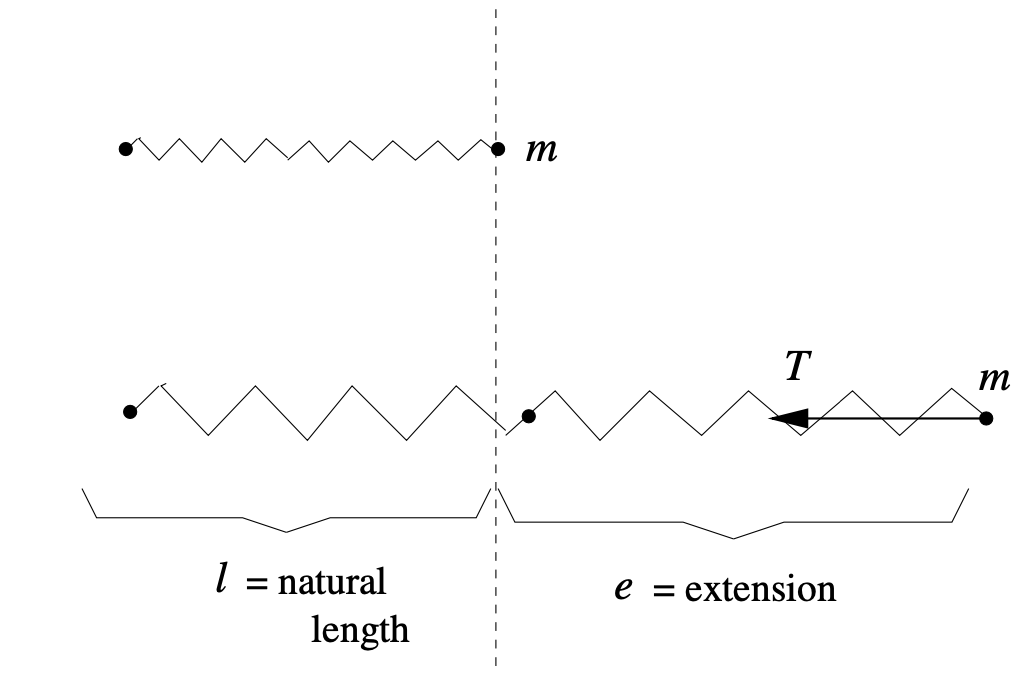
0.3.4 Contact Forces
The forces due to the contact of two objects are called contact forces.
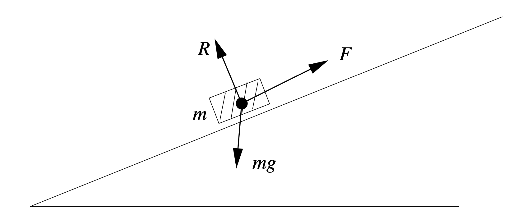
Where is the normal force, %22%2F%3E%3C%2Fg%3E%3C%2Fg%3E%3Cdefs%3E%3Csymbol%20id%3D%22a%22%20overflow%3D%22visible%22%3E%3Cpath%20d%3D%22M2.985%209.84c0-.15.165-.225.48-.225.6%200%20.9-.06.9-.195%200-.045-.03-.15-.075-.345L2.34%201.23C2.25.9%202.1.705%201.89.63%201.785.6%201.515.585%201.05.585.72.585.57.555.57.24.57.075.66%200%20.855%200l1.95.045L5.025%200c.24%200%20.36.12.36.345%200%20.255-.165.24-.555.24-.66%200-1.035.03-1.125.105-.045.015-.06.075-.06.15l.96%203.975H6c.69%200%201.17-.03%201.17-.6%200-.195-.03-.435-.105-.72a3%203%200%200%201-.045-.165c0-.165.075-.24.24-.24.075.015.18.12.285.345l.81%203.225c.03.12.045.21.045.255-.045.135-.135.21-.24.21-.12%200-.21-.12-.27-.345-.15-.57-.36-.93-.6-1.11q-.36-.27-1.26-.27H4.755l.93%203.69c.12.51.12.525.75.525h1.95c1.455%200%202.115-.225%202.115-1.56%200-.3-.015-.57-.045-.795-.015-.165-.03-.255-.03-.27%200-.165.075-.24.225-.24s.24.135.27.42l.3%202.565c.045.42-.06.465-.465.465h-7.26c-.345%200-.51-.015-.51-.36%22%2F%3E%3C%2Fsymbol%3E%3C%2Fdefs%3E%3C%2Fsvg%3E) is the frictional force.
is the frictional force.
0.3.4.1 Moving Friction
Given a moving object on a surface with coefficient of kinetic friction %22%2F%3E%3Cuse%20xlink%3Ahref%3D%22%23b%22%20class%3D%22typst-text%22%20transform%3D%22matrix(1%200%200%20-1%2010.045%2011.335)%22%2F%3E%3C%2Fg%3E%3C%2Fg%3E%3Cdefs%3E%3Csymbol%20id%3D%22a%22%20overflow%3D%22visible%22%3E%3Cpath%20d%3D%22M8.58%202.13c0%20.135-.075.21-.24.21-.12%200-.21-.105-.255-.3-.3-1.2-.66-1.8-1.065-1.8-.255%200-.39.21-.39.63%200%20.255.09.765.285%201.515l.42%201.605c.135.54.255.915.345%201.38l.09.42c.03.105.045.18.045.21%200%20.315-.165.465-.495.465s-.54-.18-.63-.555L5.61%201.62c0-.165-.24-.465-.72-.915A1.6%201.6%200%200%200%203.75.24c-.69%200-1.035.405-1.035%201.23%200%20.285.06.69.195%201.245l.63%202.49c.12.465.195.795.225.96%200%20.315-.165.465-.495.465s-.54-.195-.645-.585l-2.13-8.58a1.2%201.2%200%200%201-.045-.24c0-.315.165-.465.48-.465.225%200%20.405.12.57.345.045.105.3%201.14.795%203.105q.54-.405%201.395-.405c.885%200%201.47.465%201.935%201.005A1.39%201.39%200%200%201%206.99-.195c1.035%200%201.35%201.215%201.59%202.325%22%2F%3E%3C%2Fsymbol%3E%3Csymbol%20id%3D%22b%22%20overflow%3D%22visible%22%3E%3Cpath%20d%3D%22M5.954%203.896c0%20.462-.378.766-.84.766-.473%200-1.03-.304-1.68-.924-.473-.451-.851-.745-1.114-.872L3.33%206.92c.01.02.02.083.041.178%200%20.126-.073.189-.21.189l-1.323-.105c-.178-.01-.262-.105-.262-.284%200-.115.105-.178.305-.178.178%200%20.462%200%20.462-.115a.8.8%200%200%200-.042-.221C1.795%204.378%201.313%202.352.798.357.788.315.788.283.788.273c0-.252.125-.378.388-.378.262%200%20.43.157.515.462.167.64.409%201.596.504%201.985.829-.095%201.249-.358%201.249-.809%200-.095-.063-.43-.063-.525%200-.651.494-1.113%201.134-1.113.378%200%20.693.189.934.567.221.347.357.693.42%201.06%200%20.116-.073.179-.21.179a.24.24%200%200%201-.136-.032.8.8%200%200%201-.105-.252C5.208.652%204.914.274%204.546.274c-.21%200-.315.168-.315.493%200%20.126.022.274.053.452.032.115.053.22.053.336%200%20.452-.232.767-.704.924a4%204%200%200%201-.882.21c.2.136.451.346.756.62.493.44.956.976%201.596.976.115%200%20.2-.021.263-.063-.326-.084-.494-.284-.494-.609%200-.252.2-.43.452-.43.378%200%20.63.336.63.714%22%2F%3E%3C%2Fsymbol%3E%3C%2Fdefs%3E%3C%2Fsvg%3E) ,
and normal force acting on the object,
the frictional force
,
and normal force acting on the object,
the frictional force %22%2F%3E%3Cuse%20xlink%3Ahref%3D%22%23b%22%20class%3D%22typst-text%22%20transform%3D%22matrix(1%200%200%20-1%208.995%2014.905)%22%2F%3E%3C%2Fg%3E%3C%2Fg%3E%3Cdefs%3E%3Csymbol%20id%3D%22a%22%20overflow%3D%22visible%22%3E%3Cpath%20d%3D%22M2.985%209.84c0-.15.165-.225.48-.225.6%200%20.9-.06.9-.195%200-.045-.03-.15-.075-.345L2.34%201.23C2.25.9%202.1.705%201.89.63%201.785.6%201.515.585%201.05.585.72.585.57.555.57.24.57.075.66%200%20.855%200l1.95.045L5.025%200c.24%200%20.36.12.36.345%200%20.255-.165.24-.555.24-.66%200-1.035.03-1.125.105-.045.015-.06.075-.06.15l.96%203.975H6c.69%200%201.17-.03%201.17-.6%200-.195-.03-.435-.105-.72a3%203%200%200%201-.045-.165c0-.165.075-.24.24-.24.075.015.18.12.285.345l.81%203.225c.03.12.045.21.045.255-.045.135-.135.21-.24.21-.12%200-.21-.12-.27-.345-.15-.57-.36-.93-.6-1.11q-.36-.27-1.26-.27H4.755l.93%203.69c.12.51.12.525.75.525h1.95c1.455%200%202.115-.225%202.115-1.56%200-.3-.015-.57-.045-.795-.015-.165-.03-.255-.03-.27%200-.165.075-.24.225-.24s.24.135.27.42l.3%202.565c.045.42-.06.465-.465.465h-7.26c-.345%200-.51-.015-.51-.36%22%2F%3E%3C%2Fsymbol%3E%3Csymbol%20id%3D%22b%22%20overflow%3D%22visible%22%3E%3Cpath%20d%3D%22M5.954%203.896c0%20.462-.378.766-.84.766-.473%200-1.03-.304-1.68-.924-.473-.451-.851-.745-1.114-.872L3.33%206.92c.01.02.02.083.041.178%200%20.126-.073.189-.21.189l-1.323-.105c-.178-.01-.262-.105-.262-.284%200-.115.105-.178.305-.178.178%200%20.462%200%20.462-.115a.8.8%200%200%200-.042-.221C1.795%204.378%201.313%202.352.798.357.788.315.788.283.788.273c0-.252.125-.378.388-.378.262%200%20.43.157.515.462.167.64.409%201.596.504%201.985.829-.095%201.249-.358%201.249-.809%200-.095-.063-.43-.063-.525%200-.651.494-1.113%201.134-1.113.378%200%20.693.189.934.567.221.347.357.693.42%201.06%200%20.116-.073.179-.21.179a.24.24%200%200%201-.136-.032.8.8%200%200%201-.105-.252C5.208.652%204.914.274%204.546.274c-.21%200-.315.168-.315.493%200%20.126.022.274.053.452.032.115.053.22.053.336%200%20.452-.232.767-.704.924a4%204%200%200%201-.882.21c.2.136.451.346.756.62.493.44.956.976%201.596.976.115%200%20.2-.021.263-.063-.326-.084-.494-.284-.494-.609%200-.252.2-.43.452-.43.378%200%20.63.336.63.714%22%2F%3E%3C%2Fsymbol%3E%3C%2Fdefs%3E%3C%2Fsvg%3E) acting on the object is given by:
acting on the object is given by:
%22%2F%3E%3Cuse%20xlink%3Ahref%3D%22%23b%22%20class%3D%22typst-text%22%20transform%3D%22matrix(1%200%200%20-1%2017.995%2023.95)%22%2F%3E%3Cuse%20xlink%3Ahref%3D%22%23c%22%20class%3D%22typst-text%22%20transform%3D%22matrix(1%200%200%20-1%2029.375%2020.245)%22%2F%3E%3Cuse%20xlink%3Ahref%3D%22%23d%22%20class%3D%22typst-text%22%20transform%3D%22matrix(1%200%200%20-1%2045.212%2020.245)%22%2F%3E%3Cuse%20xlink%3Ahref%3D%22%23e%22%20class%3D%22typst-text%22%20transform%3D%22matrix(1%200%200%20-1%2056.882%2020.245)%22%2F%3E%3Cuse%20xlink%3Ahref%3D%22%23b%22%20class%3D%22typst-text%22%20transform%3D%22matrix(1%200%200%20-1%2065.927%2023.95)%22%2F%3E%3Cuse%20xlink%3Ahref%3D%22%23f%22%20class%3D%22typst-text%22%20transform%3D%22matrix(1%200%200%20-1%2073.14%2020.245)%22%2F%3E%3C%2Fg%3E%3C%2Fg%3E%3Cdefs%3E%3Csymbol%20id%3D%22a%22%20overflow%3D%22visible%22%3E%3Cpath%20d%3D%22M2.985%209.84c0-.15.165-.225.48-.225.6%200%20.9-.06.9-.195%200-.045-.03-.15-.075-.345L2.34%201.23C2.25.9%202.1.705%201.89.63%201.785.6%201.515.585%201.05.585.72.585.57.555.57.24.57.075.66%200%20.855%200l1.95.045L5.025%200c.24%200%20.36.12.36.345%200%20.255-.165.24-.555.24-.66%200-1.035.03-1.125.105-.045.015-.06.075-.06.15l.96%203.975H6c.69%200%201.17-.03%201.17-.6%200-.195-.03-.435-.105-.72a3%203%200%200%201-.045-.165c0-.165.075-.24.24-.24.075.015.18.12.285.345l.81%203.225c.03.12.045.21.045.255-.045.135-.135.21-.24.21-.12%200-.21-.12-.27-.345-.15-.57-.36-.93-.6-1.11q-.36-.27-1.26-.27H4.755l.93%203.69c.12.51.12.525.75.525h1.95c1.455%200%202.115-.225%202.115-1.56%200-.3-.015-.57-.045-.795-.015-.165-.03-.255-.03-.27%200-.165.075-.24.225-.24s.24.135.27.42l.3%202.565c.045.42-.06.465-.465.465h-7.26c-.345%200-.51-.015-.51-.36%22%2F%3E%3C%2Fsymbol%3E%3Csymbol%20id%3D%22b%22%20overflow%3D%22visible%22%3E%3Cpath%20d%3D%22M5.954%203.896c0%20.462-.378.766-.84.766-.473%200-1.03-.304-1.68-.924-.473-.451-.851-.745-1.114-.872L3.33%206.92c.01.02.02.083.041.178%200%20.126-.073.189-.21.189l-1.323-.105c-.178-.01-.262-.105-.262-.284%200-.115.105-.178.305-.178.178%200%20.462%200%20.462-.115a.8.8%200%200%200-.042-.221C1.795%204.378%201.313%202.352.798.357.788.315.788.283.788.273c0-.252.125-.378.388-.378.262%200%20.43.157.515.462.167.64.409%201.596.504%201.985.829-.095%201.249-.358%201.249-.809%200-.095-.063-.43-.063-.525%200-.651.494-1.113%201.134-1.113.378%200%20.693.189.934.567.221.347.357.693.42%201.06%200%20.116-.073.179-.21.179a.24.24%200%200%201-.136-.032.8.8%200%200%201-.105-.252C5.208.652%204.914.274%204.546.274c-.21%200-.315.168-.315.493%200%20.126.022.274.053.452.032.115.053.22.053.336%200%20.452-.232.767-.704.924a4%204%200%200%201-.882.21c.2.136.451.346.756.62.493.44.956.976%201.596.976.115%200%20.2-.021.263-.063-.326-.084-.494-.284-.494-.609%200-.252.2-.43.452-.43.378%200%20.63.336.63.714%22%2F%3E%3C%2Fsymbol%3E%3Csymbol%20id%3D%22c%22%20overflow%3D%22visible%22%3E%3Cpath%20d%3D%22M10.47%205.505H1.2c-.24%200-.36-.12-.36-.345s.12-.345.36-.345h9.27c.24%200%20.36.12.36.345%200%20.18-.165.345-.36.345m0-2.82H1.2c-.24%200-.36-.12-.36-.345s.12-.345.36-.345h9.27c.24%200%20.36.12.36.345a.35.35%200%200%201-.36.345%22%2F%3E%3C%2Fsymbol%3E%3Csymbol%20id%3D%22d%22%20overflow%3D%22visible%22%3E%3Cpath%20d%3D%22M10.47%204.05H1.2c-.24%200-.36-.105-.36-.3s.12-.3.36-.3h9.27c.24%200%20.36.105.36.3%200%20.18-.18.3-.36.3%22%2F%3E%3C%2Fsymbol%3E%3Csymbol%20id%3D%22e%22%20overflow%3D%22visible%22%3E%3Cpath%20d%3D%22M8.58%202.13c0%20.135-.075.21-.24.21-.12%200-.21-.105-.255-.3-.3-1.2-.66-1.8-1.065-1.8-.255%200-.39.21-.39.63%200%20.255.09.765.285%201.515l.42%201.605c.135.54.255.915.345%201.38l.09.42c.03.105.045.18.045.21%200%20.315-.165.465-.495.465s-.54-.18-.63-.555L5.61%201.62c0-.165-.24-.465-.72-.915A1.6%201.6%200%200%200%203.75.24c-.69%200-1.035.405-1.035%201.23%200%20.285.06.69.195%201.245l.63%202.49c.12.465.195.795.225.96%200%20.315-.165.465-.495.465s-.54-.195-.645-.585l-2.13-8.58a1.2%201.2%200%200%201-.045-.24c0-.315.165-.465.48-.465.225%200%20.405.12.57.345.045.105.3%201.14.795%203.105q.54-.405%201.395-.405c.885%200%201.47.465%201.935%201.005A1.39%201.39%200%200%201%206.99-.195c1.035%200%201.35%201.215%201.59%202.325%22%2F%3E%3C%2Fsymbol%3E%3Csymbol%20id%3D%22f%22%20overflow%3D%22visible%22%3E%3Cpath%20d%3D%22M11.085%207.965c0%20.765-.39%201.35-1.155%201.77-.615.345-1.35.51-2.175.51h-4.23c-.345%200-.495-.015-.495-.36%200-.105.045-.18.135-.195.15-.015.27-.03.345-.03.45-.015.705-.045.78-.06s.12-.06.12-.135c0-.03-.015-.12-.06-.27L2.37%201.23C2.295.9%202.145.69%201.92.615%201.815.585%201.545.57%201.08.57.75.57.615.555.615.225q0-.247.27-.225l1.86.045L4.635%200c.24-.015.36.12.36.345%200%20.15-.165.225-.48.225-.6%200-.9.075-.9.21%200%200%20.015.03.045.24l.96%203.885h1.725c1.035%200%201.56-.435%201.56-1.29%200-.135-.075-.465-.21-1.005-.165-.63-.24-1.05-.24-1.275C7.455.195%208.34-.33%209.48-.33c.42%200%20.825.195%201.23.57s.615.78.615%201.2c0%20.15-.075.225-.24.225-.105%200-.195-.075-.24-.24C10.68.96%2010.47.615%2010.23.42s-.465-.3-.69-.3c-.345%200-.525.285-.525.84%200%20.36.045.915.15%201.68.045.315.06.54.06.705%200%20.795-.42%201.38-1.26%201.74%201.41.345%203.12%201.35%203.12%202.88M9.135%209.24q.45-.293.45-.99c0-.3-.06-.645-.195-1.05q-.607-1.845-3.06-1.845H4.74l.945%203.795q.113.472.36.495c.075.015.375.015.9.015.975%200%201.545-.03%202.19-.42%22%2F%3E%3C%2Fsymbol%3E%3C%2Fdefs%3E%3C%2Fsvg%3E)
0.4 Work and Energy
0.4.1 Potential Energy
Given a particle of mass and position vector ,
the potential energy %22%2F%3E%3C%2Fg%3E%3C%2Fg%3E%3Cdefs%3E%3Csymbol%20id%3D%22a%22%20overflow%3D%22visible%22%3E%3Cpath%20d%3D%22M9.63%2010.2c-.285%200-1.245.045-1.53.045-.225%200-.33-.12-.33-.36q0-.202.315-.225c.645%200%20.96-.195.96-.585%200-.09-.015-.195-.045-.3L7.665%203.48A4.73%204.73%200%200%200%206.36%201.26C5.655.585%204.875.255%204.035.255c-1.11%200-1.755.75-1.755%201.86l.015.135c0%20.285.045.615.15%201.005l1.44%205.775q.112.472.405.585c.09.03.345.045.78.045.39%200%20.555%200%20.555.36%200%20.15-.09.225-.255.225L3.465%2010.2l-1.905.045c-.24%200-.345-.135-.345-.36%200-.105.045-.18.12-.195.15-.015.27-.03.345-.03.465-.015.735-.045.81-.06s.105-.06.105-.135c0-.03-.015-.135-.06-.3L1.11%203.45a3.4%203.4%200%200%201-.105-.87c0-1.725%201.245-2.91%202.97-2.91.975%200%201.875.375%202.7%201.14.795.72%201.305%201.56%201.545%202.535L9.54%208.61c.195.765.615%201.035%201.545%201.05q.315.023.315.36v.06c-.045.105-.12.165-.255.165-.285%200-1.23-.045-1.515-.045%22%2F%3E%3C%2Fsymbol%3E%3C%2Fdefs%3E%3C%2Fsvg%3E) of the particle is given by:
of the particle is given by:
%22%2F%3E%3Cuse%20xlink%3Ahref%3D%22%23b%22%20class%3D%22typst-text%22%20transform%3D%22matrix(1%200%200%20-1%2025.987%2021.22)%22%2F%3E%3Cuse%20xlink%3Ahref%3D%22%23a%22%20class%3D%22typst-text%22%20transform%3D%22matrix(1%200%200%20-1%2041.823%2021.22)%22%2F%3E%3Cuse%20xlink%3Ahref%3D%22%23c%22%20class%3D%22typst-text%22%20transform%3D%22matrix(1%200%200%20-1%2053.643%2021.22)%22%2F%3E%3Cuse%20xlink%3Ahref%3D%22%23d%22%20class%3D%22typst-text%22%20transform%3D%22matrix(1%200%200%20-1%2059.478%2021.22)%22%2F%3E%3Cuse%20xlink%3Ahref%3D%22%23e%22%20class%3D%22typst-text%22%20transform%3D%22matrix(1%200%200%20-1%2066.588%2021.22)%22%2F%3E%3C%2Fg%3E%3C%2Fg%3E%3Cdefs%3E%3Csymbol%20id%3D%22a%22%20overflow%3D%22visible%22%3E%3Cpath%20d%3D%22M9.63%2010.2c-.285%200-1.245.045-1.53.045-.225%200-.33-.12-.33-.36q0-.202.315-.225c.645%200%20.96-.195.96-.585%200-.09-.015-.195-.045-.3L7.665%203.48A4.73%204.73%200%200%200%206.36%201.26C5.655.585%204.875.255%204.035.255c-1.11%200-1.755.75-1.755%201.86l.015.135c0%20.285.045.615.15%201.005l1.44%205.775q.112.472.405.585c.09.03.345.045.78.045.39%200%20.555%200%20.555.36%200%20.15-.09.225-.255.225L3.465%2010.2l-1.905.045c-.24%200-.345-.135-.345-.36%200-.105.045-.18.12-.195.15-.015.27-.03.345-.03.465-.015.735-.045.81-.06s.105-.06.105-.135c0-.03-.015-.135-.06-.3L1.11%203.45a3.4%203.4%200%200%201-.105-.87c0-1.725%201.245-2.91%202.97-2.91.975%200%201.875.375%202.7%201.14.795.72%201.305%201.56%201.545%202.535L9.54%208.61c.195.765.615%201.035%201.545%201.05q.315.023.315.36v.06c-.045.105-.12.165-.255.165-.285%200-1.23-.045-1.515-.045%22%2F%3E%3C%2Fsymbol%3E%3Csymbol%20id%3D%22b%22%20overflow%3D%22visible%22%3E%3Cpath%20d%3D%22M10.47%205.505H1.2c-.24%200-.36-.12-.36-.345s.12-.345.36-.345h9.27c.24%200%20.36.12.36.345%200%20.18-.165.345-.36.345m0-2.82H1.2c-.24%200-.36-.12-.36-.345s.12-.345.36-.345h9.27c.24%200%20.36.12.36.345a.35.35%200%200%201-.36.345%22%2F%3E%3C%2Fsymbol%3E%3Csymbol%20id%3D%22c%22%20overflow%3D%22visible%22%3E%3Cpath%20d%3D%22M4.77-3.72c.135%200%20.21.075.21.21%200%20.045-.03.105-.075.165-.78.6-1.41%201.59-1.875%202.955-.405%201.185-.615%202.355-.615%203.51v1.26c0%201.155.21%202.325.615%203.51.465%201.365%201.095%202.355%201.875%202.955a.24.24%200%200%201%20.075.165c0%20.135-.075.21-.21.21a.3.3%200%200%201-.105-.045c-.9-.69-1.65-1.71-2.265-3.075-.585-1.305-.885-2.535-.885-3.72V3.12c0-1.185.3-2.415.885-3.72.615-1.365%201.365-2.385%202.265-3.075a.3.3%200%200%201%20.105-.045%22%2F%3E%3C%2Fsymbol%3E%3Csymbol%20id%3D%22d%22%20overflow%3D%22visible%22%3E%3Cpath%20d%3D%22M6.63%205.52c0%20.795-.81%201.23-1.59%201.23-1.05%200-1.65-.75-1.995-1.695V6.75l-2.49-.12v-.705c.93%200%201.035%200%201.035-.585V.705H.555V0l1.89.045c.57%200%201.53%200%202.07-.045v.705H3.21V3.33c0%201.05.375%202.88%201.875%202.88%200%200-.285-.255-.285-.69%200-.615.48-.915.915-.915s.915.315.915.915%22%2F%3E%3C%2Fsymbol%3E%3Csymbol%20id%3D%22e%22%20overflow%3D%22visible%22%3E%3Cpath%20d%3D%22M1.17-3.675c.9.69%201.65%201.71%202.265%203.075.585%201.305.885%202.535.885%203.72v1.26c0%201.185-.3%202.415-.885%203.72-.615%201.365-1.365%202.385-2.265%203.075a.3.3%200%200%201-.105.045c-.135%200-.21-.075-.21-.21%200-.06.03-.12.075-.165.78-.6%201.41-1.59%201.875-2.955.405-1.185.615-2.355.615-3.51V3.12c0-1.155-.21-2.325-.615-3.51C2.34-1.755%201.71-2.745.93-3.345c-.045-.06-.075-.12-.075-.165%200-.135.075-.21.21-.21.015%200%20.06.015.105.045%22%2F%3E%3C%2Fsymbol%3E%3C%2Fdefs%3E%3C%2Fsvg%3E)
and the force acting on the particle is given by:
%22%2F%3E%3Cuse%20xlink%3Ahref%3D%22%23b%22%20class%3D%22typst-text%22%20transform%3D%22matrix(1%200%200%20-1%2025.027%2020.245)%22%2F%3E%3Cuse%20xlink%3Ahref%3D%22%23c%22%20class%3D%22typst-text%22%20transform%3D%22matrix(1%200%200%20-1%2040.863%2020.245)%22%2F%3E%3Cuse%20xlink%3Ahref%3D%22%23d%22%20class%3D%22typst-text%22%20transform%3D%22matrix(1%200%200%20-1%2052.533%2020.245)%22%2F%3E%3Cuse%20xlink%3Ahref%3D%22%23e%22%20class%3D%22typst-text%22%20transform%3D%22matrix(1%200%200%20-1%2065.028%2020.245)%22%2F%3E%3C%2Fg%3E%3C%2Fg%3E%3Cdefs%3E%3Csymbol%20id%3D%22a%22%20overflow%3D%22visible%22%3E%3Cpath%20d%3D%22M10.125%206.585%209.66%2010.2H.585v-.705h1.62V.705H.585V0c.57.045%202.085.045%202.745.045.735%200%202.37%200%203.03-.045v.705H4.335v4.05h.75C6.525%204.755%206.66%204.11%206.66%203h.705v4.215H6.66c0-1.11-.12-1.755-1.575-1.755h-.75v4.035h2.1c2.415%200%202.76-1.155%202.985-2.91Z%22%2F%3E%3C%2Fsymbol%3E%3Csymbol%20id%3D%22b%22%20overflow%3D%22visible%22%3E%3Cpath%20d%3D%22M10.47%205.505H1.2c-.24%200-.36-.12-.36-.345s.12-.345.36-.345h9.27c.24%200%20.36.12.36.345%200%20.18-.165.345-.36.345m0-2.82H1.2c-.24%200-.36-.12-.36-.345s.12-.345.36-.345h9.27c.24%200%20.36.12.36.345a.35.35%200%200%201-.36.345%22%2F%3E%3C%2Fsymbol%3E%3Csymbol%20id%3D%22c%22%20overflow%3D%22visible%22%3E%3Cpath%20d%3D%22M10.47%204.05H1.2c-.24%200-.36-.105-.36-.3s.12-.3.36-.3h9.27c.24%200%20.36.105.36.3%200%20.18-.18.3-.36.3%22%2F%3E%3C%2Fsymbol%3E%3Csymbol%20id%3D%22d%22%20overflow%3D%22visible%22%3E%3Cpath%20d%3D%22M11.7%209.855a1%201%200%200%201%20.075.21c0%20.12-.135.18-.39.18H1.095c-.255%200-.39-.06-.39-.195l5.1-10.245c.105-.195.24-.3.435-.3s.33.105.435.3ZM6.675%201.08l-3.99%207.995h7.965Z%22%2F%3E%3C%2Fsymbol%3E%3Csymbol%20id%3D%22e%22%20overflow%3D%22visible%22%3E%3Cpath%20d%3D%22M9.63%2010.2c-.285%200-1.245.045-1.53.045-.225%200-.33-.12-.33-.36q0-.202.315-.225c.645%200%20.96-.195.96-.585%200-.09-.015-.195-.045-.3L7.665%203.48A4.73%204.73%200%200%200%206.36%201.26C5.655.585%204.875.255%204.035.255c-1.11%200-1.755.75-1.755%201.86l.015.135c0%20.285.045.615.15%201.005l1.44%205.775q.112.472.405.585c.09.03.345.045.78.045.39%200%20.555%200%20.555.36%200%20.15-.09.225-.255.225L3.465%2010.2l-1.905.045c-.24%200-.345-.135-.345-.36%200-.105.045-.18.12-.195.15-.015.27-.03.345-.03.465-.015.735-.045.81-.06s.105-.06.105-.135c0-.03-.015-.135-.06-.3L1.11%203.45a3.4%203.4%200%200%201-.105-.87c0-1.725%201.245-2.91%202.97-2.91.975%200%201.875.375%202.7%201.14.795.72%201.305%201.56%201.545%202.535L9.54%208.61c.195.765.615%201.035%201.545%201.05q.315.023.315.36v.06c-.045.105-.12.165-.255.165-.285%200-1.23-.045-1.515-.045%22%2F%3E%3C%2Fsymbol%3E%3C%2Fdefs%3E%3C%2Fsvg%3E)
Consequently, the potential energy can be expressed in terms of the force acting on the particle:
%22%2F%3E%3Cuse%20xlink%3Ahref%3D%22%23b%22%20class%3D%22typst-text%22%20transform%3D%22matrix(1%200%200%20-1%2025.987%2030.415)%22%2F%3E%3Cuse%20xlink%3Ahref%3D%22%23c%22%20class%3D%22typst-text%22%20transform%3D%22matrix(1%200%200%20-1%2041.823%2030.415)%22%2F%3E%3Cuse%20xlink%3Ahref%3D%22%23d%22%20class%3D%22typst-text%22%20transform%3D%22matrix(1%200%200%20-1%2055.993%2030.415)%22%2F%3E%3Cuse%20xlink%3Ahref%3D%22%23e%22%20class%3D%22typst-text%22%20transform%3D%22matrix(1%200%200%20-1%2073.478%2030.415)%22%2F%3E%3Cuse%20xlink%3Ahref%3D%22%23f%22%20class%3D%22typst-text%22%20transform%3D%22matrix(1%200%200%20-1%2087.672%2030.415)%22%2F%3E%3Cuse%20xlink%3Ahref%3D%22%23g%22%20class%3D%22typst-text%22%20transform%3D%22matrix(1%200%200%20-1%2095.175%2030.415)%22%2F%3E%3Cuse%20xlink%3Ahref%3D%22%23h%22%20class%3D%22typst-text%22%20transform%3D%22matrix(1%200%200%20-1%20103.335%2030.415)%22%2F%3E%3C%2Fg%3E%3C%2Fg%3E%3Cdefs%3E%3Csymbol%20id%3D%22a%22%20overflow%3D%22visible%22%3E%3Cpath%20d%3D%22M9.63%2010.2c-.285%200-1.245.045-1.53.045-.225%200-.33-.12-.33-.36q0-.202.315-.225c.645%200%20.96-.195.96-.585%200-.09-.015-.195-.045-.3L7.665%203.48A4.73%204.73%200%200%200%206.36%201.26C5.655.585%204.875.255%204.035.255c-1.11%200-1.755.75-1.755%201.86l.015.135c0%20.285.045.615.15%201.005l1.44%205.775q.112.472.405.585c.09.03.345.045.78.045.39%200%20.555%200%20.555.36%200%20.15-.09.225-.255.225L3.465%2010.2l-1.905.045c-.24%200-.345-.135-.345-.36%200-.105.045-.18.12-.195.15-.015.27-.03.345-.03.465-.015.735-.045.81-.06s.105-.06.105-.135c0-.03-.015-.135-.06-.3L1.11%203.45a3.4%203.4%200%200%201-.105-.87c0-1.725%201.245-2.91%202.97-2.91.975%200%201.875.375%202.7%201.14.795.72%201.305%201.56%201.545%202.535L9.54%208.61c.195.765.615%201.035%201.545%201.05q.315.023.315.36v.06c-.045.105-.12.165-.255.165-.285%200-1.23-.045-1.515-.045%22%2F%3E%3C%2Fsymbol%3E%3Csymbol%20id%3D%22b%22%20overflow%3D%22visible%22%3E%3Cpath%20d%3D%22M10.47%205.505H1.2c-.24%200-.36-.12-.36-.345s.12-.345.36-.345h9.27c.24%200%20.36.12.36.345%200%20.18-.165.345-.36.345m0-2.82H1.2c-.24%200-.36-.12-.36-.345s.12-.345.36-.345h9.27c.24%200%20.36.12.36.345a.35.35%200%200%201-.36.345%22%2F%3E%3C%2Fsymbol%3E%3Csymbol%20id%3D%22c%22%20overflow%3D%22visible%22%3E%3Cpath%20d%3D%22M10.47%204.05H1.2c-.24%200-.36-.105-.36-.3s.12-.3.36-.3h9.27c.24%200%20.36.105.36.3%200%20.18-.18.3-.36.3%22%2F%3E%3C%2Fsymbol%3E%3Csymbol%20id%3D%22d%22%20overflow%3D%22visible%22%3E%3Cpath%20d%3D%22M12.465%2020.415c-.705%200-1.335-.645-1.92-1.935-.285-.615-.585-1.545-.915-2.79C8.175%2010.32%207.08%205.085%205.925-1.755%205.4-4.92%204.965-7.215%204.62-8.61c-.615-2.565-1.32-3.855-2.1-3.855-.285%200-.54.075-.765.24.435.075.645.33.645.78%200%20.435-.33.78-.765.78-.525%200-.795-.27-.795-.795%200-.87.855-1.455%201.71-1.455%201.095%200%201.995.87%202.7%202.595.375.915.885%202.685%201.515%205.28C7.86-.585%208.835%204.185%209.69%209.255c.6%203.555%201.14%206.255%201.605%208.1.435%201.74.84%202.61%201.2%202.61.3%200%20.555-.075.75-.24-.435-.075-.66-.33-.66-.78%200-.435.33-.78.765-.78.525%200%20.795.27.795.795%200%20.825-.81%201.455-1.68%201.455%22%2F%3E%3C%2Fsymbol%3E%3Csymbol%20id%3D%22e%22%20overflow%3D%22visible%22%3E%3Cpath%20d%3D%22M10.125%206.585%209.66%2010.2H.585v-.705h1.62V.705H.585V0c.57.045%202.085.045%202.745.045.735%200%202.37%200%203.03-.045v.705H4.335v4.05h.75C6.525%204.755%206.66%204.11%206.66%203h.705v4.215H6.66c0-1.11-.12-1.755-1.575-1.755h-.75v4.035h2.1c2.415%200%202.76-1.155%202.985-2.91Z%22%2F%3E%3C%2Fsymbol%3E%3Csymbol%20id%3D%22f%22%20overflow%3D%22visible%22%3E%3Cpath%20d%3D%22M2.88%203.75a.8.8%200%200%201-.795.795.8.8%200%200%201-.795-.795.8.8%200%200%201%20.795-.795.8.8%200%200%201%20.795.795%22%2F%3E%3C%2Fsymbol%3E%3Csymbol%20id%3D%22g%22%20overflow%3D%22visible%22%3E%3Cpath%20d%3D%22M6.435%209.48%205.55%205.835c-.315.555-.75.84-1.335.84-.975%200-1.83-.495-2.58-1.5C.945%204.245.6%203.27.6%202.265c0-1.32.765-2.43%202.025-2.43C3.27-.165%203.9.18%204.5.885c.165-.57.675-1.05%201.38-1.05%201.035%200%201.365%201.23%201.59%202.34%200%20.135-.075.21-.225.21q-.202%200-.27-.315C6.675.885%206.315.285%205.91.285c-.255%200-.39.21-.39.615%200%20.225.03.465.09.705l2.13%208.58v.06a.26.26%200%200%201-.255.165c-.345%200-.975-.06-1.875-.165-.165-.015-.255-.135-.255-.345q0-.225.405-.225c.285%200%20.675.015.675-.195m-1.32-3.84c.15-.315.225-.525.225-.66a2%202%200%200%201-.045-.24L4.56%201.83a1.7%201.7%200%200%200-.285-.525C3.72.63%203.18.285%202.655.285c-.585%200-.885.45-.885%201.335q0%20.54.27%201.62c.315%201.275.765%202.145%201.32%202.61.3.255.585.375.87.375.405%200%20.705-.195.885-.585%22%2F%3E%3C%2Fsymbol%3E%3Csymbol%20id%3D%22h%22%20overflow%3D%22visible%22%3E%3Cpath%20d%3D%22M6.63%205.52c0%20.795-.81%201.23-1.59%201.23-1.05%200-1.65-.75-1.995-1.695V6.75l-2.49-.12v-.705c.93%200%201.035%200%201.035-.585V.705H.555V0l1.89.045c.57%200%201.53%200%202.07-.045v.705H3.21V3.33c0%201.05.375%202.88%201.875%202.88%200%200-.285-.255-.285-.69%200-.615.48-.915.915-.915s.915.315.915.915%22%2F%3E%3C%2Fsymbol%3E%3C%2Fdefs%3E%3C%2Fsvg%3E)
0.4.2 Energy Conservation
Given a particle of mass and position vector ,
the total energy %22%2F%3E%3C%2Fg%3E%3C%2Fg%3E%3Cdefs%3E%3Csymbol%20id%3D%22a%22%20overflow%3D%22visible%22%3E%3Cpath%20d%3D%22M2.985%209.84c0-.15.165-.225.48-.225.6%200%20.9-.06.9-.195%200-.045-.03-.15-.075-.345L2.34%201.23C2.265.9%202.115.705%201.89.63%201.785.6%201.515.585%201.05.585.72.585.57.555.57.24.57.075.735%200%201.05%200h7.695c.36%200%20.39.03.51.285l.6%201.35c.405.93.69%201.62.855%202.085-.03.135-.075.225-.24.225-.105%200-.195-.075-.255-.21-.375-.885-.735-1.56-1.095-2.04-.6-.81-1.485-1.11-2.895-1.11H4.05c-.15%200-.255%200-.315.015-.09%200-.135.03-.135.075%200%20.03.03.135.075.33l.99%204.005H6.09c.705%200%201.08-.09%201.155-.285a.9.9%200%200%200%20.045-.33c0-.195-.03-.435-.105-.72a.5.5%200%200%201-.045-.18c0-.15.09-.225.255-.225.135%200%20.225.12.285.345l.84%203.48c0%20.15-.075.225-.24.225-.12%200-.21-.105-.255-.315-.15-.585-.345-.96-.6-1.14s-.675-.27-1.29-.27h-1.32l.87%203.495c.12.51.12.525.75.525H8.52q1.148%200%201.575-.225.63-.338.63-1.35c0-.255-.015-.525-.06-.78%200-.03%200-.075-.015-.135V6.99c0-.165.075-.24.225-.24s.24.135.27.42l.3%202.565c.045.42-.06.465-.465.465H3.495c-.345%200-.51-.015-.51-.36%22%2F%3E%3C%2Fsymbol%3E%3C%2Fdefs%3E%3C%2Fsvg%3E) of the particle is given by:
of the particle is given by:
%22%2F%3E%3Cuse%20xlink%3Ahref%3D%22%23b%22%20class%3D%22typst-text%22%20transform%3D%22matrix(1%200%200%20-1%2026.047%2020.245)%22%2F%3E%3Cuse%20xlink%3Ahref%3D%22%23c%22%20class%3D%22typst-text%22%20transform%3D%22matrix(1%200%200%20-1%2041.883%2020.245)%22%2F%3E%3Cuse%20xlink%3Ahref%3D%22%23d%22%20class%3D%22typst-text%22%20transform%3D%22matrix(1%200%200%20-1%2056.197%2020.245)%22%2F%3E%3Cuse%20xlink%3Ahref%3D%22%23e%22%20class%3D%22typst-text%22%20transform%3D%22matrix(1%200%200%20-1%2071.2%2020.245)%22%2F%3E%3C%2Fg%3E%3C%2Fg%3E%3Cdefs%3E%3Csymbol%20id%3D%22a%22%20overflow%3D%22visible%22%3E%3Cpath%20d%3D%22M2.985%209.84c0-.15.165-.225.48-.225.6%200%20.9-.06.9-.195%200-.045-.03-.15-.075-.345L2.34%201.23C2.265.9%202.115.705%201.89.63%201.785.6%201.515.585%201.05.585.72.585.57.555.57.24.57.075.735%200%201.05%200h7.695c.36%200%20.39.03.51.285l.6%201.35c.405.93.69%201.62.855%202.085-.03.135-.075.225-.24.225-.105%200-.195-.075-.255-.21-.375-.885-.735-1.56-1.095-2.04-.6-.81-1.485-1.11-2.895-1.11H4.05c-.15%200-.255%200-.315.015-.09%200-.135.03-.135.075%200%20.03.03.135.075.33l.99%204.005H6.09c.705%200%201.08-.09%201.155-.285a.9.9%200%200%200%20.045-.33c0-.195-.03-.435-.105-.72a.5.5%200%200%201-.045-.18c0-.15.09-.225.255-.225.135%200%20.225.12.285.345l.84%203.48c0%20.15-.075.225-.24.225-.12%200-.21-.105-.255-.315-.15-.585-.345-.96-.6-1.14s-.675-.27-1.29-.27h-1.32l.87%203.495c.12.51.12.525.75.525H8.52q1.148%200%201.575-.225.63-.338.63-1.35c0-.255-.015-.525-.06-.78%200-.03%200-.075-.015-.135V6.99c0-.165.075-.24.225-.24s.24.135.27.42l.3%202.565c.045.42-.06.465-.465.465H3.495c-.345%200-.51-.015-.51-.36%22%2F%3E%3C%2Fsymbol%3E%3Csymbol%20id%3D%22b%22%20overflow%3D%22visible%22%3E%3Cpath%20d%3D%22M10.47%205.505H1.2c-.24%200-.36-.12-.36-.345s.12-.345.36-.345h9.27c.24%200%20.36.12.36.345%200%20.18-.165.345-.36.345m0-2.82H1.2c-.24%200-.36-.12-.36-.345s.12-.345.36-.345h9.27c.24%200%20.36.12.36.345a.35.35%200%200%201-.36.345%22%2F%3E%3C%2Fsymbol%3E%3Csymbol%20id%3D%22c%22%20overflow%3D%22visible%22%3E%3Cpath%20d%3D%22M5.16%209.465c0-.045-.015-.15-.06-.3l-1.98-7.92c-.06-.225-.12-.36-.165-.42C2.82.66%202.31.585%201.41.585.945.585.735.63.735.24c0-.165.105-.24.3-.24.765%200%201.845.06%202.49.045L4.755.03C4.965.03%205.79%200%206.045%200s.375.12.375.36c0%20.15-.18.225-.555.225-.78%200-1.23.03-1.365.105-.045.03-.075.09-.075.18L6.45%209.045c.045.21.09.345.135.39q.09.135%201.08.135c.825%200%201.395-.06%201.68-.195s.435-.45.435-.96c0-.27-.045-.66-.12-1.17-.03-.12-.045-.21-.045-.285%200-.165.075-.255.24-.255.135%200%20.225.135.27.39l.405%202.58c.015.075.03.165.03.255%200%20.15-.15.225-.465.225h-8.22c-.39%200-.42-.045-.54-.33L.45%207.215a5%205%200%200%201-.09-.285c0-.15.075-.225.24-.225.12%200%20.225.12.3.345.375%201.095.75%201.77%201.095%202.055.39.315%201.14.465%202.235.465h.585c.165%200%20.345.015.345-.105%22%2F%3E%3C%2Fsymbol%3E%3Csymbol%20id%3D%22d%22%20overflow%3D%22visible%22%3E%3Cpath%20d%3D%22M10.47%204.11H6.195v4.275q0%20.36-.36.36t-.36-.36V4.11H1.2q-.36%200-.36-.36t.36-.36h4.275V-.885q0-.36.36-.36t.36.36V3.39h4.275q.36%200%20.36.36c0%20.195-.165.36-.36.36%22%2F%3E%3C%2Fsymbol%3E%3Csymbol%20id%3D%22e%22%20overflow%3D%22visible%22%3E%3Cpath%20d%3D%22M9.63%2010.2c-.285%200-1.245.045-1.53.045-.225%200-.33-.12-.33-.36q0-.202.315-.225c.645%200%20.96-.195.96-.585%200-.09-.015-.195-.045-.3L7.665%203.48A4.73%204.73%200%200%200%206.36%201.26C5.655.585%204.875.255%204.035.255c-1.11%200-1.755.75-1.755%201.86l.015.135c0%20.285.045.615.15%201.005l1.44%205.775q.112.472.405.585c.09.03.345.045.78.045.39%200%20.555%200%20.555.36%200%20.15-.09.225-.255.225L3.465%2010.2l-1.905.045c-.24%200-.345-.135-.345-.36%200-.105.045-.18.12-.195.15-.015.27-.03.345-.03.465-.015.735-.045.81-.06s.105-.06.105-.135c0-.03-.015-.135-.06-.3L1.11%203.45a3.4%203.4%200%200%201-.105-.87c0-1.725%201.245-2.91%202.97-2.91.975%200%201.875.375%202.7%201.14.795.72%201.305%201.56%201.545%202.535L9.54%208.61c.195.765.615%201.035%201.545%201.05q.315.023.315.36v.06c-.045.105-.12.165-.255.165-.285%200-1.23-.045-1.515-.045%22%2F%3E%3C%2Fsymbol%3E%3C%2Fdefs%3E%3C%2Fsvg%3E)
where is the kinetic energy of the particle,
and is the potential energy of the particle.
If the net external force acting on the particle is zero, then the total energy of the particle is conserved:

0.4.2.1 Conservative Forces
Given a force acting on a particle,
if the force is conservative, then the force can be expressed as the gradient of a scalar function:
where is the potential energy of the particle.
For conservative forces, on a simply connected domain (the domain is path connected and any closed curve can be shrunk to a point without leaving the domain),
the work done by the force on the particle is path independent:

0.4.2.1.1 Example: Non-conservative Forces
Given a force acting on a particle,
where the force can be expressed as:
%22%2F%3E%3Cuse%20xlink%3Ahref%3D%22%23b%22%20class%3D%22typst-text%22%20transform%3D%22matrix(1%200%200%20-1%2020.86%2021.22)%22%2F%3E%3Cuse%20xlink%3Ahref%3D%22%23c%22%20class%3D%22typst-text%22%20transform%3D%22matrix(1%200%200%20-1%2026.695%2021.22)%22%2F%3E%3Cuse%20xlink%3Ahref%3D%22%23d%22%20class%3D%22typst-text%22%20transform%3D%22matrix(1%200%200%20-1%2035.275%2021.22)%22%2F%3E%3Cuse%20xlink%3Ahref%3D%22%23e%22%20class%3D%22typst-text%22%20transform%3D%22matrix(1%200%200%20-1%2041.945%2021.22)%22%2F%3E%3Cuse%20xlink%3Ahref%3D%22%23d%22%20class%3D%22typst-text%22%20transform%3D%22matrix(1%200%200%20-1%2049.715%2021.22)%22%2F%3E%3Cuse%20xlink%3Ahref%3D%22%23f%22%20class%3D%22typst-text%22%20transform%3D%22matrix(1%200%200%20-1%2056.385%2021.22)%22%2F%3E%3Cuse%20xlink%3Ahref%3D%22%23g%22%20class%3D%22typst-text%22%20transform%3D%22matrix(1%200%200%20-1%2063.81%2021.22)%22%2F%3E%3Cuse%20xlink%3Ahref%3D%22%23h%22%20class%3D%22typst-text%22%20transform%3D%22matrix(1%200%200%20-1%2073.812%2021.22)%22%2F%3E%3Cuse%20xlink%3Ahref%3D%22%23b%22%20class%3D%22typst-text%22%20transform%3D%22matrix(1%200%200%20-1%2089.648%2021.22)%22%2F%3E%3Cuse%20xlink%3Ahref%3D%22%23i%22%20class%3D%22typst-text%22%20transform%3D%22matrix(1%200%200%20-1%2095.483%2021.22)%22%2F%3E%3Cuse%20xlink%3Ahref%3D%22%23d%22%20class%3D%22typst-text%22%20transform%3D%22matrix(1%200%200%20-1%20102.983%2021.22)%22%2F%3E%3Cuse%20xlink%3Ahref%3D%22%23i%22%20class%3D%22typst-text%22%20transform%3D%22matrix(1%200%200%20-1%20109.653%2021.22)%22%2F%3E%3Cuse%20xlink%3Ahref%3D%22%23d%22%20class%3D%22typst-text%22%20transform%3D%22matrix(1%200%200%20-1%20117.153%2021.22)%22%2F%3E%3Cuse%20xlink%3Ahref%3D%22%23c%22%20class%3D%22typst-text%22%20transform%3D%22matrix(1%200%200%20-1%20123.823%2021.22)%22%2F%3E%3Cuse%20xlink%3Ahref%3D%22%23g%22%20class%3D%22typst-text%22%20transform%3D%22matrix(1%200%200%20-1%20132.403%2021.22)%22%2F%3E%3C%2Fg%3E%3C%2Fg%3E%3Cdefs%3E%3Csymbol%20id%3D%22a%22%20overflow%3D%22visible%22%3E%3Cpath%20d%3D%22M10.125%206.585%209.66%2010.2H.585v-.705h1.62V.705H.585V0c.57.045%202.085.045%202.745.045.735%200%202.37%200%203.03-.045v.705H4.335v4.05h.75C6.525%204.755%206.66%204.11%206.66%203h.705v4.215H6.66c0-1.11-.12-1.755-1.575-1.755h-.75v4.035h2.1c2.415%200%202.76-1.155%202.985-2.91Z%22%2F%3E%3C%2Fsymbol%3E%3Csymbol%20id%3D%22b%22%20overflow%3D%22visible%22%3E%3Cpath%20d%3D%22M4.77-3.72c.135%200%20.21.075.21.21%200%20.045-.03.105-.075.165-.78.6-1.41%201.59-1.875%202.955-.405%201.185-.615%202.355-.615%203.51v1.26c0%201.155.21%202.325.615%203.51.465%201.365%201.095%202.355%201.875%202.955a.24.24%200%200%201%20.075.165c0%20.135-.075.21-.21.21a.3.3%200%200%201-.105-.045c-.9-.69-1.65-1.71-2.265-3.075-.585-1.305-.885-2.535-.885-3.72V3.12c0-1.185.3-2.415.885-3.72.615-1.365%201.365-2.385%202.265-3.075a.3.3%200%200%201%20.105-.045%22%2F%3E%3C%2Fsymbol%3E%3Csymbol%20id%3D%22c%22%20overflow%3D%22visible%22%3E%3Cpath%20d%3D%22M7.905%205.595c0%20.69-.675%201.035-1.425%201.035-.645%200-1.155-.345-1.545-1.035-.315.69-.84%201.035-1.605%201.035-.735%200-1.335-.345-1.815-1.02C1.11%205.025.9%204.59.9%204.305c0-.135.075-.21.225-.21.135%200%20.225.075.255.21.285.87.915%201.89%201.92%201.89.495%200%20.735-.315.735-.93%200-.315-.27-1.485-.795-3.495C2.985.765%202.535.27%201.89.27c-.21%200-.405.045-.57.12q.585.225.585.81c0%20.39-.195.585-.6.585-.495%200-.87-.42-.87-.915%200-.69.705-1.035%201.44-1.035.63%200%201.14.345%201.545%201.035.285-.69.825-1.035%201.605-1.035.72%200%201.32.345%201.8%201.02.405.585.615%201.02.615%201.305%200%20.135-.075.21-.225.21-.135%200-.21-.075-.255-.21C6.705%201.305%206.03.27%205.055.27c-.495%200-.75.3-.75.915%200%20.195.075.615.24%201.29l.51%202.025c.285%201.125.75%201.695%201.41%201.695.21%200%20.405-.045.57-.12-.405-.135-.6-.405-.6-.81%200-.39.21-.585.615-.585.48%200%20.855.435.855.915%22%2F%3E%3C%2Fsymbol%3E%3Csymbol%20id%3D%22d%22%20overflow%3D%22visible%22%3E%3Cpath%20d%3D%22M2.085%201.59c-.48%200-.795-.36-.795-.84%200-.45.345-.825.795-.825.21%200%20.39.06.525.195L2.625%200c0-.945-.315-1.755-.945-2.4-.105-.12-.165-.21-.165-.27%200-.15.06-.225.195-.225s.315.18.57.525c.51.72.765%201.515.765%202.37%200%20.795-.27%201.59-.96%201.59%22%2F%3E%3C%2Fsymbol%3E%3Csymbol%20id%3D%22e%22%20overflow%3D%22visible%22%3E%3Cpath%20d%3D%22M2.445%206.63Q1.432%206.63.87%205.505C.585%204.92.435%204.515.435%204.29c0-.135.075-.21.24-.21.21%200%20.225.09.285.315.345%201.185.825%201.785%201.44%201.785.195%200%20.3-.135.3-.405%200-.24-.075-.585-.24-1.02-.57-1.545-.855-2.58-.855-3.135%200-1.14.705-1.815%201.86-1.815.495%200%20.96.18%201.38.54q-.788-2.97-2.475-2.97-.765%200-1.035.495.9.045.9.855c0%20.375-.195.57-.6.57-.555%200-.885-.465-.885-1.02%200-.825.75-1.35%201.62-1.35%201.725%200%203.135%201.59%203.51%203.06l1.41%205.67c.045.165.06.285.06.36%200%20.3-.165.45-.48.45-.24%200-.435-.12-.57-.345-.09-.315-.165-.585-.21-.81l-.96-3.855C4.98.915%204.185.24%203.51.24c-.57%200-.855.375-.855%201.14%200%20.63.255%201.59.75%202.88.195.525.3.885.3%201.095%200%20.735-.525%201.275-1.26%201.275%22%2F%3E%3C%2Fsymbol%3E%3Csymbol%20id%3D%22f%22%20overflow%3D%22visible%22%3E%3Cpath%20d%3D%22m2.43%201.38-.255-.03c.72.705%201.275%201.215%201.65%201.56l1.44%201.335c.345.315.705.705%201.05%201.14.465.57.69.915.69%201.035%200%20.135-.075.21-.225.21-.105%200-.195-.06-.27-.195-.375-.615-.72-.915-1.05-.915s-.57.27-.705.45c-.36.435-.72.66-1.065.66-.39%200-.795-.18-1.215-.57q-.63-.585-.63-1.17c0-.15.075-.225.24-.225.105%200%20.195.075.255.21.165.435.57.645%201.185.645.21%200%20.51-.075.915-.21.36-.135.705-.21%201.02-.225a47%2047%200%200%200-1.95-1.83L2.175%202.01a14%2014%200%200%201-.825-.9C.885.525.645.18.645.045s.075-.21.24-.21c.09%200%20.18.075.285.225.375.585.78.885%201.2.885.24%200%20.51-.18.81-.555s.645-.555.99-.555c.51%200%201.02.27%201.56.795q.81.788.81%201.53c0%20.135-.075.21-.24.21q-.158%200-.27-.225a1.81%201.81%200%200%200-1.71-1.2c-.36%200-1.53.435-1.89.435%22%2F%3E%3C%2Fsymbol%3E%3Csymbol%20id%3D%22g%22%20overflow%3D%22visible%22%3E%3Cpath%20d%3D%22M1.17-3.675c.9.69%201.65%201.71%202.265%203.075.585%201.305.885%202.535.885%203.72v1.26c0%201.185-.3%202.415-.885%203.72-.615%201.365-1.365%202.385-2.265%203.075a.3.3%200%200%201-.105.045c-.135%200-.21-.075-.21-.21%200-.06.03-.12.075-.165.78-.6%201.41-1.59%201.875-2.955.405-1.185.615-2.355.615-3.51V3.12c0-1.155-.21-2.325-.615-3.51C2.34-1.755%201.71-2.745.93-3.345c-.045-.06-.075-.12-.075-.165%200-.135.075-.21.21-.21.015%200%20.06.015.105.045%22%2F%3E%3C%2Fsymbol%3E%3Csymbol%20id%3D%22h%22%20overflow%3D%22visible%22%3E%3Cpath%20d%3D%22M10.47%205.505H1.2c-.24%200-.36-.12-.36-.345s.12-.345.36-.345h9.27c.24%200%20.36.12.36.345%200%20.18-.165.345-.36.345m0-2.82H1.2c-.24%200-.36-.12-.36-.345s.12-.345.36-.345h9.27c.24%200%20.36.12.36.345a.35.35%200%200%201-.36.345%22%2F%3E%3C%2Fsymbol%3E%3Csymbol%20id%3D%22i%22%20overflow%3D%22visible%22%3E%3Cpath%20d%3D%22M3.735-.33C5.85-.33%206.9%201.38%206.9%204.8c0%202.295-.48%203.825-1.425%204.575-.525.405-1.11.615-1.725.615C1.635%209.99.585%208.265.585%204.8c0-2.76.735-5.13%203.15-5.13m1.68%208.19c.105-.525.15-1.485.15-2.88%200-1.38-.06-2.4-.165-3.06Q5.107.12%203.735.12c-.345%200-.69.135-1.005.39-.405.345-.645%201.05-.75%202.13-.045.375-.06%201.155-.06%202.34%200%201.305.045%202.22.12%202.715.135.825.405%201.35.825%201.575.33.18.615.27.87.27.975%200%201.515-.795%201.68-1.68%22%2F%3E%3C%2Fsymbol%3E%3C%2Fdefs%3E%3C%2Fsvg%3E)
by solving the PDE, there is no potential energy such that:
Thus, the force is non-conservative.
0.4.2.1.2 Essential Conditions for Conservative Forces
Given a force acting on a particle,
the force is conservative if the following conditions are satisfied:
-
The force
is a function of the position vector only. -
The force
is irrotational, that is, the curl of the force is zero:%22%2F%3E%3Cuse%20xlink%3Ahref%3D%22%23b%22%20class%3D%22typst-text%22%20transform%3D%22matrix(1%200%200%20-1%2025.828%2020.245)%22%2F%3E%3Cuse%20xlink%3Ahref%3D%22%23c%22%20class%3D%22typst-text%22%20transform%3D%22matrix(1%200%200%20-1%2040.832%2020.245)%22%2F%3E%3Cuse%20xlink%3Ahref%3D%22%23d%22%20class%3D%22typst-text%22%20transform%3D%22matrix(1%200%200%20-1%2055.858%2020.245)%22%2F%3E%3Cuse%20xlink%3Ahref%3D%22%23e%22%20class%3D%22typst-text%22%20transform%3D%22matrix(1%200%200%20-1%2071.695%2020.245)%22%2F%3E%3C%2Fg%3E%3C%2Fg%3E%3Cdefs%3E%3Csymbol%20id%3D%22a%22%20overflow%3D%22visible%22%3E%3Cpath%20d%3D%22M11.7%209.855a1%201%200%200%201%20.075.21c0%20.12-.135.18-.39.18H1.095c-.255%200-.39-.06-.39-.195l5.1-10.245c.105-.195.24-.3.435-.3s.33.105.435.3ZM6.675%201.08l-3.99%207.995h7.965Z%22%2F%3E%3C%2Fsymbol%3E%3Csymbol%20id%3D%22b%22%20overflow%3D%22visible%22%3E%3Cpath%20d%3D%22M9.45.48c0%20.105-.03.18-.105.255L6.33%203.75l3.015%203.015c.075.075.105.15.105.255a.34.34%200%200%201-.345.345.33.33%200%200%201-.255-.105L5.835%204.245%202.82%207.26a.33.33%200%200%201-.255.105.34.34%200%200%201-.345-.345c0-.105.03-.18.105-.255L5.34%203.75%202.325.735A.33.33%200%200%201%202.22.48a.34.34%200%200%201%20.345-.345c.105%200%20.18.03.255.105l3.015%203.015L8.85.24a.33.33%200%200%201%20.255-.105.34.34%200%200%201%20.345.345%22%2F%3E%3C%2Fsymbol%3E%3Csymbol%20id%3D%22c%22%20overflow%3D%22visible%22%3E%3Cpath%20d%3D%22M10.125%206.585%209.66%2010.2H.585v-.705h1.62V.705H.585V0c.57.045%202.085.045%202.745.045.735%200%202.37%200%203.03-.045v.705H4.335v4.05h.75C6.525%204.755%206.66%204.11%206.66%203h.705v4.215H6.66c0-1.11-.12-1.755-1.575-1.755h-.75v4.035h2.1c2.415%200%202.76-1.155%202.985-2.91Z%22%2F%3E%3C%2Fsymbol%3E%3Csymbol%20id%3D%22d%22%20overflow%3D%22visible%22%3E%3Cpath%20d%3D%22M10.47%205.505H1.2c-.24%200-.36-.12-.36-.345s.12-.345.36-.345h9.27c.24%200%20.36.12.36.345%200%20.18-.165.345-.36.345m0-2.82H1.2c-.24%200-.36-.12-.36-.345s.12-.345.36-.345h9.27c.24%200%20.36.12.36.345a.35.35%200%200%201-.36.345%22%2F%3E%3C%2Fsymbol%3E%3Csymbol%20id%3D%22e%22%20overflow%3D%22visible%22%3E%3Cpath%20d%3D%22M3.735-.33C5.85-.33%206.9%201.38%206.9%204.8c0%202.295-.48%203.825-1.425%204.575-.525.405-1.11.615-1.725.615C1.635%209.99.585%208.265.585%204.8c0-2.76.735-5.13%203.15-5.13m1.68%208.19c.105-.525.15-1.485.15-2.88%200-1.38-.06-2.4-.165-3.06Q5.107.12%203.735.12c-.345%200-.69.135-1.005.39-.405.345-.645%201.05-.75%202.13-.045.375-.06%201.155-.06%202.34%200%201.305.045%202.22.12%202.715.135.825.405%201.35.825%201.575.33.18.615.27.87.27.975%200%201.515-.795%201.68-1.68%22%2F%3E%3C%2Fsymbol%3E%3C%2Fdefs%3E%3C%2Fsvg%3E)
0.4.2.2 Qualitative Energy Analysis
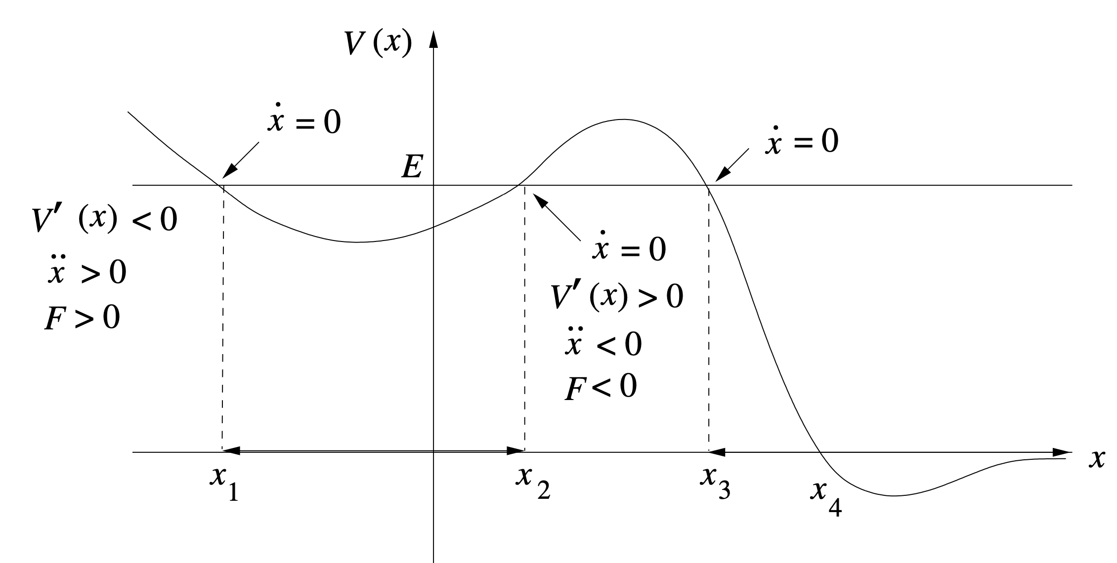
At point %22%2F%3E%3Cuse%20xlink%3Ahref%3D%22%23b%22%20class%3D%22typst-text%22%20transform%3D%22matrix(1%200%200%20-1%209.58%2011.335)%22%2F%3E%3C%2Fg%3E%3C%2Fg%3E%3Cdefs%3E%3Csymbol%20id%3D%22a%22%20overflow%3D%22visible%22%3E%3Cpath%20d%3D%22M7.905%205.595c0%20.69-.675%201.035-1.425%201.035-.645%200-1.155-.345-1.545-1.035-.315.69-.84%201.035-1.605%201.035-.735%200-1.335-.345-1.815-1.02C1.11%205.025.9%204.59.9%204.305c0-.135.075-.21.225-.21.135%200%20.225.075.255.21.285.87.915%201.89%201.92%201.89.495%200%20.735-.315.735-.93%200-.315-.27-1.485-.795-3.495C2.985.765%202.535.27%201.89.27c-.21%200-.405.045-.57.12q.585.225.585.81c0%20.39-.195.585-.6.585-.495%200-.87-.42-.87-.915%200-.69.705-1.035%201.44-1.035.63%200%201.14.345%201.545%201.035.285-.69.825-1.035%201.605-1.035.72%200%201.32.345%201.8%201.02.405.585.615%201.02.615%201.305%200%20.135-.075.21-.225.21-.135%200-.21-.075-.255-.21C6.705%201.305%206.03.27%205.055.27c-.495%200-.75.3-.75.915%200%20.195.075.615.24%201.29l.51%202.025c.285%201.125.75%201.695%201.41%201.695.21%200%20.405-.045.57-.12-.405-.135-.6-.405-.6-.81%200-.39.21-.585.615-.585.48%200%20.855.435.855.915%22%2F%3E%3C%2Fsymbol%3E%3Csymbol%20id%3D%22b%22%20overflow%3D%22visible%22%3E%3Cpath%20d%3D%22M3.182%206.972c-.452-.441-1.124-.662-2.037-.662v-.46c.619%200%201.112.094%201.49.272V.894c0-.137-.01-.221-.041-.263q-.08-.176-.945-.178h-.431V0l1.869.042L4.967%200v.452h-.431q-.864.002-.955.178c-.022.042-.032.126-.032.262v5.744c0%20.284-.042.336-.367.336%22%2F%3E%3C%2Fsymbol%3E%3C%2Fdefs%3E%3C%2Fsvg%3E) ,
the particle has speed
,
the particle has speed %22%2F%3E%3Cuse%20xlink%3Ahref%3D%22%23b%22%20class%3D%22typst-text%22%20transform%3D%22matrix(1%200%200%20-1%201%2011.035)%22%2F%3E%3Cuse%20xlink%3Ahref%3D%22%23c%22%20class%3D%22typst-text%22%20transform%3D%22matrix(1%200%200%20-1%2013.747%2011.035)%22%2F%3E%3Cuse%20xlink%3Ahref%3D%22%23d%22%20class%3D%22typst-text%22%20transform%3D%22matrix(1%200%200%20-1%2029.583%2011.035)%22%2F%3E%3C%2Fg%3E%3C%2Fg%3E%3Cdefs%3E%3Csymbol%20id%3D%22a%22%20overflow%3D%22visible%22%3E%3Cpath%20d%3D%22M-3.165%209.36a.8.8%200%200%201-.795.795.813.813%200%200%201-.81-.795.8.8%200%200%201%20.795-.795c.435%200%20.81.36.81.795%22%2F%3E%3C%2Fsymbol%3E%3Csymbol%20id%3D%22b%22%20overflow%3D%22visible%22%3E%3Cpath%20d%3D%22M7.905%205.595c0%20.69-.675%201.035-1.425%201.035-.645%200-1.155-.345-1.545-1.035-.315.69-.84%201.035-1.605%201.035-.735%200-1.335-.345-1.815-1.02C1.11%205.025.9%204.59.9%204.305c0-.135.075-.21.225-.21.135%200%20.225.075.255.21.285.87.915%201.89%201.92%201.89.495%200%20.735-.315.735-.93%200-.315-.27-1.485-.795-3.495C2.985.765%202.535.27%201.89.27c-.21%200-.405.045-.57.12q.585.225.585.81c0%20.39-.195.585-.6.585-.495%200-.87-.42-.87-.915%200-.69.705-1.035%201.44-1.035.63%200%201.14.345%201.545%201.035.285-.69.825-1.035%201.605-1.035.72%200%201.32.345%201.8%201.02.405.585.615%201.02.615%201.305%200%20.135-.075.21-.225.21-.135%200-.21-.075-.255-.21C6.705%201.305%206.03.27%205.055.27c-.495%200-.75.3-.75.915%200%20.195.075.615.24%201.29l.51%202.025c.285%201.125.75%201.695%201.41%201.695.21%200%20.405-.045.57-.12-.405-.135-.6-.405-.6-.81%200-.39.21-.585.615-.585.48%200%20.855.435.855.915%22%2F%3E%3C%2Fsymbol%3E%3Csymbol%20id%3D%22c%22%20overflow%3D%22visible%22%3E%3Cpath%20d%3D%22M10.47%205.505H1.2c-.24%200-.36-.12-.36-.345s.12-.345.36-.345h9.27c.24%200%20.36.12.36.345%200%20.18-.165.345-.36.345m0-2.82H1.2c-.24%200-.36-.12-.36-.345s.12-.345.36-.345h9.27c.24%200%20.36.12.36.345a.35.35%200%200%201-.36.345%22%2F%3E%3C%2Fsymbol%3E%3Csymbol%20id%3D%22d%22%20overflow%3D%22visible%22%3E%3Cpath%20d%3D%22M3.735-.33C5.85-.33%206.9%201.38%206.9%204.8c0%202.295-.48%203.825-1.425%204.575-.525.405-1.11.615-1.725.615C1.635%209.99.585%208.265.585%204.8c0-2.76.735-5.13%203.15-5.13m1.68%208.19c.105-.525.15-1.485.15-2.88%200-1.38-.06-2.4-.165-3.06Q5.107.12%203.735.12c-.345%200-.69.135-1.005.39-.405.345-.645%201.05-.75%202.13-.045.375-.06%201.155-.06%202.34%200%201.305.045%202.22.12%202.715.135.825.405%201.35.825%201.575.33.18.615.27.87.27.975%200%201.515-.795%201.68-1.68%22%2F%3E%3C%2Fsymbol%3E%3C%2Fdefs%3E%3C%2Fsvg%3E) and potential energy
and potential energy %22%2F%3E%3Cuse%20xlink%3Ahref%3D%22%23b%22%20class%3D%22typst-text%22%20transform%3D%22matrix(1%200%200%20-1%2012.955%2012.22)%22%2F%3E%3Cuse%20xlink%3Ahref%3D%22%23c%22%20class%3D%22typst-text%22%20transform%3D%22matrix(1%200%200%20-1%2017.62%2012.22)%22%2F%3E%3Cuse%20xlink%3Ahref%3D%22%23d%22%20class%3D%22typst-text%22%20transform%3D%22matrix(1%200%200%20-1%2023.455%2012.22)%22%2F%3E%3Cuse%20xlink%3Ahref%3D%22%23e%22%20class%3D%22typst-text%22%20transform%3D%22matrix(1%200%200%20-1%2032.035%2012.22)%22%2F%3E%3Cuse%20xlink%3Ahref%3D%22%23f%22%20class%3D%22typst-text%22%20transform%3D%22matrix(1%200%200%20-1%2042.037%2012.22)%22%2F%3E%3Cuse%20xlink%3Ahref%3D%22%23g%22%20class%3D%22typst-text%22%20transform%3D%22matrix(1%200%200%20-1%2057.873%2012.22)%22%2F%3E%3C%2Fg%3E%3C%2Fg%3E%3Cdefs%3E%3Csymbol%20id%3D%22a%22%20overflow%3D%22visible%22%3E%3Cpath%20d%3D%22M10.065%2010.2c-.285%200-1.185.045-1.47.045-.225%200-.345-.12-.345-.345%200-.15.105-.225.3-.24.42-.015.63-.165.63-.42%200-.135-.075-.315-.21-.54L4.5%201.605l-.99%207.68c0%20.255.315.375.96.375.3%200%20.435.105.435.36q0%20.225-.27.225c-.33%200-1.5-.045-1.83-.045-.3%200-1.32.045-1.62.045-.225%200-.345-.12-.345-.345%200-.165.15-.24.435-.24.255%200%20.435-.03.555-.06.24-.075.225-.105.27-.39L3.27.06c.045-.255.165-.39.36-.39s.345.105.465.3l5.34%208.49c.345.54.675.885%201.005%201.02.225.105.51.165.84.18.165.015.24.12.255.345.015.165-.075.24-.255.24-.225%200-.99-.045-1.215-.045%22%2F%3E%3C%2Fsymbol%3E%3Csymbol%20id%3D%22b%22%20overflow%3D%22visible%22%3E%3Cpath%20d%3D%22M3.165%2011.22a.56.56%200%200%201-.54-.345L.87%206.45h.51l2.295%203.84q.09.113.09.315c0%20.33-.255.615-.6.615%22%2F%3E%3C%2Fsymbol%3E%3Csymbol%20id%3D%22c%22%20overflow%3D%22visible%22%3E%3Cpath%20d%3D%22M4.77-3.72c.135%200%20.21.075.21.21%200%20.045-.03.105-.075.165-.78.6-1.41%201.59-1.875%202.955-.405%201.185-.615%202.355-.615%203.51v1.26c0%201.155.21%202.325.615%203.51.465%201.365%201.095%202.355%201.875%202.955a.24.24%200%200%201%20.075.165c0%20.135-.075.21-.21.21a.3.3%200%200%201-.105-.045c-.9-.69-1.65-1.71-2.265-3.075-.585-1.305-.885-2.535-.885-3.72V3.12c0-1.185.3-2.415.885-3.72.615-1.365%201.365-2.385%202.265-3.075a.3.3%200%200%201%20.105-.045%22%2F%3E%3C%2Fsymbol%3E%3Csymbol%20id%3D%22d%22%20overflow%3D%22visible%22%3E%3Cpath%20d%3D%22M7.905%205.595c0%20.69-.675%201.035-1.425%201.035-.645%200-1.155-.345-1.545-1.035-.315.69-.84%201.035-1.605%201.035-.735%200-1.335-.345-1.815-1.02C1.11%205.025.9%204.59.9%204.305c0-.135.075-.21.225-.21.135%200%20.225.075.255.21.285.87.915%201.89%201.92%201.89.495%200%20.735-.315.735-.93%200-.315-.27-1.485-.795-3.495C2.985.765%202.535.27%201.89.27c-.21%200-.405.045-.57.12q.585.225.585.81c0%20.39-.195.585-.6.585-.495%200-.87-.42-.87-.915%200-.69.705-1.035%201.44-1.035.63%200%201.14.345%201.545%201.035.285-.69.825-1.035%201.605-1.035.72%200%201.32.345%201.8%201.02.405.585.615%201.02.615%201.305%200%20.135-.075.21-.225.21-.135%200-.21-.075-.255-.21C6.705%201.305%206.03.27%205.055.27c-.495%200-.75.3-.75.915%200%20.195.075.615.24%201.29l.51%202.025c.285%201.125.75%201.695%201.41%201.695.21%200%20.405-.045.57-.12-.405-.135-.6-.405-.6-.81%200-.39.21-.585.615-.585.48%200%20.855.435.855.915%22%2F%3E%3C%2Fsymbol%3E%3Csymbol%20id%3D%22e%22%20overflow%3D%22visible%22%3E%3Cpath%20d%3D%22M1.17-3.675c.9.69%201.65%201.71%202.265%203.075.585%201.305.885%202.535.885%203.72v1.26c0%201.185-.3%202.415-.885%203.72-.615%201.365-1.365%202.385-2.265%203.075a.3.3%200%200%201-.105.045c-.135%200-.21-.075-.21-.21%200-.06.03-.12.075-.165.78-.6%201.41-1.59%201.875-2.955.405-1.185.615-2.355.615-3.51V3.12c0-1.155-.21-2.325-.615-3.51C2.34-1.755%201.71-2.745.93-3.345c-.045-.06-.075-.12-.075-.165%200-.135.075-.21.21-.21.015%200%20.06.015.105.045%22%2F%3E%3C%2Fsymbol%3E%3Csymbol%20id%3D%22f%22%20overflow%3D%22visible%22%3E%3Cpath%20d%3D%22M9.99-.675c.255-.105.525.09.525.33%200%20.15-.075.255-.21.315l-8.01%203.78%208.01%203.78c.135.06.21.165.21.3%200%20.255-.12.375-.36.375a.5.5%200%200%201-.165-.03l-8.61-4.08c-.15-.075-.225-.18-.225-.345s.075-.27.225-.345Z%22%2F%3E%3C%2Fsymbol%3E%3Csymbol%20id%3D%22g%22%20overflow%3D%22visible%22%3E%3Cpath%20d%3D%22M3.735-.33C5.85-.33%206.9%201.38%206.9%204.8c0%202.295-.48%203.825-1.425%204.575-.525.405-1.11.615-1.725.615C1.635%209.99.585%208.265.585%204.8c0-2.76.735-5.13%203.15-5.13m1.68%208.19c.105-.525.15-1.485.15-2.88%200-1.38-.06-2.4-.165-3.06Q5.107.12%203.735.12c-.345%200-.69.135-1.005.39-.405.345-.645%201.05-.75%202.13-.045.375-.06%201.155-.06%202.34%200%201.305.045%202.22.12%202.715.135.825.405%201.35.825%201.575.33.18.615.27.87.27.975%200%201.515-.795%201.68-1.68%22%2F%3E%3C%2Fsymbol%3E%3C%2Fdefs%3E%3C%2Fsvg%3E) .
Thus, the particle has to move to the right.
.
Thus, the particle has to move to the right.
At point %22%2F%3E%3Cuse%20xlink%3Ahref%3D%22%23b%22%20class%3D%22typst-text%22%20transform%3D%22matrix(1%200%200%20-1%209.58%2011.335)%22%2F%3E%3C%2Fg%3E%3C%2Fg%3E%3Cdefs%3E%3Csymbol%20id%3D%22a%22%20overflow%3D%22visible%22%3E%3Cpath%20d%3D%22M7.905%205.595c0%20.69-.675%201.035-1.425%201.035-.645%200-1.155-.345-1.545-1.035-.315.69-.84%201.035-1.605%201.035-.735%200-1.335-.345-1.815-1.02C1.11%205.025.9%204.59.9%204.305c0-.135.075-.21.225-.21.135%200%20.225.075.255.21.285.87.915%201.89%201.92%201.89.495%200%20.735-.315.735-.93%200-.315-.27-1.485-.795-3.495C2.985.765%202.535.27%201.89.27c-.21%200-.405.045-.57.12q.585.225.585.81c0%20.39-.195.585-.6.585-.495%200-.87-.42-.87-.915%200-.69.705-1.035%201.44-1.035.63%200%201.14.345%201.545%201.035.285-.69.825-1.035%201.605-1.035.72%200%201.32.345%201.8%201.02.405.585.615%201.02.615%201.305%200%20.135-.075.21-.225.21-.135%200-.21-.075-.255-.21C6.705%201.305%206.03.27%205.055.27c-.495%200-.75.3-.75.915%200%20.195.075.615.24%201.29l.51%202.025c.285%201.125.75%201.695%201.41%201.695.21%200%20.405-.045.57-.12-.405-.135-.6-.405-.6-.81%200-.39.21-.585.615-.585.48%200%20.855.435.855.915%22%2F%3E%3C%2Fsymbol%3E%3Csymbol%20id%3D%22b%22%20overflow%3D%22visible%22%3E%3Cpath%20d%3D%22M1.25%204.452c.335%200%20.587.252.587.588%200%20.378-.199.577-.587.588.23.494.756.892%201.438.892.924%200%201.533-.692%201.533-1.616%200-.505-.178-.988-.546-1.46a5%205%200%200%200-.41-.504L.777.473C.64.347.661.315.661%200h4.326l.326%201.974h-.441c-.074-.556-.157-.882-.252-.955-.053-.032-.378-.053-.997-.053H1.837c.704.62%201.355%201.176%201.974%201.67.473.367.809.692%201.019.976q.473.614.473%201.292c0%20.65-.252%201.165-.767%201.543-.451.346-1.018.525-1.69.525a2.36%202.36%200%200%201-1.502-.504c-.452-.367-.683-.83-.683-1.396%200-.357.263-.62.589-.62%22%2F%3E%3C%2Fsymbol%3E%3C%2Fdefs%3E%3C%2Fsvg%3E) ,
the particle has speed and potential energy
,
the particle has speed and potential energy %22%2F%3E%3Cuse%20xlink%3Ahref%3D%22%23b%22%20class%3D%22typst-text%22%20transform%3D%22matrix(1%200%200%20-1%2012.955%2012.22)%22%2F%3E%3Cuse%20xlink%3Ahref%3D%22%23c%22%20class%3D%22typst-text%22%20transform%3D%22matrix(1%200%200%20-1%2017.62%2012.22)%22%2F%3E%3Cuse%20xlink%3Ahref%3D%22%23d%22%20class%3D%22typst-text%22%20transform%3D%22matrix(1%200%200%20-1%2023.455%2012.22)%22%2F%3E%3Cuse%20xlink%3Ahref%3D%22%23e%22%20class%3D%22typst-text%22%20transform%3D%22matrix(1%200%200%20-1%2032.035%2012.22)%22%2F%3E%3Cuse%20xlink%3Ahref%3D%22%23f%22%20class%3D%22typst-text%22%20transform%3D%22matrix(1%200%200%20-1%2042.037%2012.22)%22%2F%3E%3Cuse%20xlink%3Ahref%3D%22%23g%22%20class%3D%22typst-text%22%20transform%3D%22matrix(1%200%200%20-1%2057.873%2012.22)%22%2F%3E%3C%2Fg%3E%3C%2Fg%3E%3Cdefs%3E%3Csymbol%20id%3D%22a%22%20overflow%3D%22visible%22%3E%3Cpath%20d%3D%22M10.065%2010.2c-.285%200-1.185.045-1.47.045-.225%200-.345-.12-.345-.345%200-.15.105-.225.3-.24.42-.015.63-.165.63-.42%200-.135-.075-.315-.21-.54L4.5%201.605l-.99%207.68c0%20.255.315.375.96.375.3%200%20.435.105.435.36q0%20.225-.27.225c-.33%200-1.5-.045-1.83-.045-.3%200-1.32.045-1.62.045-.225%200-.345-.12-.345-.345%200-.165.15-.24.435-.24.255%200%20.435-.03.555-.06.24-.075.225-.105.27-.39L3.27.06c.045-.255.165-.39.36-.39s.345.105.465.3l5.34%208.49c.345.54.675.885%201.005%201.02.225.105.51.165.84.18.165.015.24.12.255.345.015.165-.075.24-.255.24-.225%200-.99-.045-1.215-.045%22%2F%3E%3C%2Fsymbol%3E%3Csymbol%20id%3D%22b%22%20overflow%3D%22visible%22%3E%3Cpath%20d%3D%22M3.165%2011.22a.56.56%200%200%201-.54-.345L.87%206.45h.51l2.295%203.84q.09.113.09.315c0%20.33-.255.615-.6.615%22%2F%3E%3C%2Fsymbol%3E%3Csymbol%20id%3D%22c%22%20overflow%3D%22visible%22%3E%3Cpath%20d%3D%22M4.77-3.72c.135%200%20.21.075.21.21%200%20.045-.03.105-.075.165-.78.6-1.41%201.59-1.875%202.955-.405%201.185-.615%202.355-.615%203.51v1.26c0%201.155.21%202.325.615%203.51.465%201.365%201.095%202.355%201.875%202.955a.24.24%200%200%201%20.075.165c0%20.135-.075.21-.21.21a.3.3%200%200%201-.105-.045c-.9-.69-1.65-1.71-2.265-3.075-.585-1.305-.885-2.535-.885-3.72V3.12c0-1.185.3-2.415.885-3.72.615-1.365%201.365-2.385%202.265-3.075a.3.3%200%200%201%20.105-.045%22%2F%3E%3C%2Fsymbol%3E%3Csymbol%20id%3D%22d%22%20overflow%3D%22visible%22%3E%3Cpath%20d%3D%22M7.905%205.595c0%20.69-.675%201.035-1.425%201.035-.645%200-1.155-.345-1.545-1.035-.315.69-.84%201.035-1.605%201.035-.735%200-1.335-.345-1.815-1.02C1.11%205.025.9%204.59.9%204.305c0-.135.075-.21.225-.21.135%200%20.225.075.255.21.285.87.915%201.89%201.92%201.89.495%200%20.735-.315.735-.93%200-.315-.27-1.485-.795-3.495C2.985.765%202.535.27%201.89.27c-.21%200-.405.045-.57.12q.585.225.585.81c0%20.39-.195.585-.6.585-.495%200-.87-.42-.87-.915%200-.69.705-1.035%201.44-1.035.63%200%201.14.345%201.545%201.035.285-.69.825-1.035%201.605-1.035.72%200%201.32.345%201.8%201.02.405.585.615%201.02.615%201.305%200%20.135-.075.21-.225.21-.135%200-.21-.075-.255-.21C6.705%201.305%206.03.27%205.055.27c-.495%200-.75.3-.75.915%200%20.195.075.615.24%201.29l.51%202.025c.285%201.125.75%201.695%201.41%201.695.21%200%20.405-.045.57-.12-.405-.135-.6-.405-.6-.81%200-.39.21-.585.615-.585.48%200%20.855.435.855.915%22%2F%3E%3C%2Fsymbol%3E%3Csymbol%20id%3D%22e%22%20overflow%3D%22visible%22%3E%3Cpath%20d%3D%22M1.17-3.675c.9.69%201.65%201.71%202.265%203.075.585%201.305.885%202.535.885%203.72v1.26c0%201.185-.3%202.415-.885%203.72-.615%201.365-1.365%202.385-2.265%203.075a.3.3%200%200%201-.105.045c-.135%200-.21-.075-.21-.21%200-.06.03-.12.075-.165.78-.6%201.41-1.59%201.875-2.955.405-1.185.615-2.355.615-3.51V3.12c0-1.155-.21-2.325-.615-3.51C2.34-1.755%201.71-2.745.93-3.345c-.045-.06-.075-.12-.075-.165%200-.135.075-.21.21-.21.015%200%20.06.015.105.045%22%2F%3E%3C%2Fsymbol%3E%3Csymbol%20id%3D%22f%22%20overflow%3D%22visible%22%3E%3Cpath%20d%3D%22M10.29%203.405c.15.075.225.18.225.345s-.075.27-.225.345l-8.61%204.08a.5.5%200%200%201-.165.03c-.24%200-.36-.12-.36-.375%200-.135.075-.24.21-.3l8.01-3.78-8.01-3.78c-.135-.06-.21-.165-.21-.3%200-.255.12-.375.36-.375.06%200%20.12.015.165.03Z%22%2F%3E%3C%2Fsymbol%3E%3Csymbol%20id%3D%22g%22%20overflow%3D%22visible%22%3E%3Cpath%20d%3D%22M3.735-.33C5.85-.33%206.9%201.38%206.9%204.8c0%202.295-.48%203.825-1.425%204.575-.525.405-1.11.615-1.725.615C1.635%209.99.585%208.265.585%204.8c0-2.76.735-5.13%203.15-5.13m1.68%208.19c.105-.525.15-1.485.15-2.88%200-1.38-.06-2.4-.165-3.06Q5.107.12%203.735.12c-.345%200-.69.135-1.005.39-.405.345-.645%201.05-.75%202.13-.045.375-.06%201.155-.06%202.34%200%201.305.045%202.22.12%202.715.135.825.405%201.35.825%201.575.33.18.615.27.87.27.975%200%201.515-.795%201.68-1.68%22%2F%3E%3C%2Fsymbol%3E%3C%2Fdefs%3E%3C%2Fsvg%3E) .
Thus, the particle has to move to the left.
.
Thus, the particle has to move to the left.
If the initial position of the particle is inside ![[x_{1},x_{2}]](data:image/svg+xml;utf8,%3Csvg%20xmlns%3D%22http%3A%2F%2Fwww.w3.org%2F2000%2Fsvg%22%20xmlns%3Axlink%3D%22http%3A%2F%2Fwww.w3.org%2F1999%2Fxlink%22%20width%3D%2263.852%22%20height%3D%2217pt%22%20class%3D%22typst-doc%22%20viewBox%3D%220%200%2047.889%2017%22%3E%3Cpath%20fill%3D%22%23fefce8%22%20d%3D%22M0%200v17h47.889V0Z%22%20class%3D%22typst-shape%22%2F%3E%3Cg%20class%3D%22typst-group%22%3E%3Cg%20class%3D%22typst-group%22%3E%3Cuse%20xlink%3Ahref%3D%22%23a%22%20class%3D%22typst-text%22%20transform%3D%22matrix(1%200%200%20-1%201%2012.25)%22%2F%3E%3Cuse%20xlink%3Ahref%3D%22%23b%22%20class%3D%22typst-text%22%20transform%3D%22matrix(1%200%200%20-1%205.26%2012.25)%22%2F%3E%3Cuse%20xlink%3Ahref%3D%22%23c%22%20class%3D%22typst-text%22%20transform%3D%22matrix(1%200%200%20-1%2013.84%2015.955)%22%2F%3E%3Cuse%20xlink%3Ahref%3D%22%23d%22%20class%3D%22typst-text%22%20transform%3D%22matrix(1%200%200%20-1%2020.654%2012.25)%22%2F%3E%3Cuse%20xlink%3Ahref%3D%22%23b%22%20class%3D%22typst-text%22%20transform%3D%22matrix(1%200%200%20-1%2027.325%2012.25)%22%2F%3E%3Cuse%20xlink%3Ahref%3D%22%23e%22%20class%3D%22typst-text%22%20transform%3D%22matrix(1%200%200%20-1%2035.904%2015.955)%22%2F%3E%3Cuse%20xlink%3Ahref%3D%22%23f%22%20class%3D%22typst-text%22%20transform%3D%22matrix(1%200%200%20-1%2042.719%2012.25)%22%2F%3E%3C%2Fg%3E%3C%2Fg%3E%3Cdefs%3E%3Csymbol%20id%3D%22a%22%20overflow%3D%22visible%22%3E%3Cpath%20d%3D%22M3.495-3.03h-1.11v13.56h1.11c.225%200%20.345.12.345.36s-.12.36-.345.36H1.71v-15h1.785c.225%200%20.345.12.345.36%200%20.18-.165.36-.345.36%22%2F%3E%3C%2Fsymbol%3E%3Csymbol%20id%3D%22b%22%20overflow%3D%22visible%22%3E%3Cpath%20d%3D%22M7.905%205.595c0%20.69-.675%201.035-1.425%201.035-.645%200-1.155-.345-1.545-1.035-.315.69-.84%201.035-1.605%201.035-.735%200-1.335-.345-1.815-1.02C1.11%205.025.9%204.59.9%204.305c0-.135.075-.21.225-.21.135%200%20.225.075.255.21.285.87.915%201.89%201.92%201.89.495%200%20.735-.315.735-.93%200-.315-.27-1.485-.795-3.495C2.985.765%202.535.27%201.89.27c-.21%200-.405.045-.57.12q.585.225.585.81c0%20.39-.195.585-.6.585-.495%200-.87-.42-.87-.915%200-.69.705-1.035%201.44-1.035.63%200%201.14.345%201.545%201.035.285-.69.825-1.035%201.605-1.035.72%200%201.32.345%201.8%201.02.405.585.615%201.02.615%201.305%200%20.135-.075.21-.225.21-.135%200-.21-.075-.255-.21C6.705%201.305%206.03.27%205.055.27c-.495%200-.75.3-.75.915%200%20.195.075.615.24%201.29l.51%202.025c.285%201.125.75%201.695%201.41%201.695.21%200%20.405-.045.57-.12-.405-.135-.6-.405-.6-.81%200-.39.21-.585.615-.585.48%200%20.855.435.855.915%22%2F%3E%3C%2Fsymbol%3E%3Csymbol%20id%3D%22c%22%20overflow%3D%22visible%22%3E%3Cpath%20d%3D%22M3.182%206.972c-.452-.441-1.124-.662-2.037-.662v-.46c.619%200%201.112.094%201.49.272V.894c0-.137-.01-.221-.041-.263q-.08-.176-.945-.178h-.431V0l1.869.042L4.967%200v.452h-.431q-.864.002-.955.178c-.022.042-.032.126-.032.262v5.744c0%20.284-.042.336-.367.336%22%2F%3E%3C%2Fsymbol%3E%3Csymbol%20id%3D%22d%22%20overflow%3D%22visible%22%3E%3Cpath%20d%3D%22M2.085%201.59c-.48%200-.795-.36-.795-.84%200-.45.345-.825.795-.825.21%200%20.39.06.525.195L2.625%200c0-.945-.315-1.755-.945-2.4-.105-.12-.165-.21-.165-.27%200-.15.06-.225.195-.225s.315.18.57.525c.51.72.765%201.515.765%202.37%200%20.795-.27%201.59-.96%201.59%22%2F%3E%3C%2Fsymbol%3E%3Csymbol%20id%3D%22e%22%20overflow%3D%22visible%22%3E%3Cpath%20d%3D%22M1.25%204.452c.335%200%20.587.252.587.588%200%20.378-.199.577-.587.588.23.494.756.892%201.438.892.924%200%201.533-.692%201.533-1.616%200-.505-.178-.988-.546-1.46a5%205%200%200%200-.41-.504L.777.473C.64.347.661.315.661%200h4.326l.326%201.974h-.441c-.074-.556-.157-.882-.252-.955-.053-.032-.378-.053-.997-.053H1.837c.704.62%201.355%201.176%201.974%201.67.473.367.809.692%201.019.976q.473.614.473%201.292c0%20.65-.252%201.165-.767%201.543-.451.346-1.018.525-1.69.525a2.36%202.36%200%200%201-1.502-.504c-.452-.367-.683-.83-.683-1.396%200-.357.263-.62.589-.62%22%2F%3E%3C%2Fsymbol%3E%3Csymbol%20id%3D%22f%22%20overflow%3D%22visible%22%3E%3Cpath%20d%3D%22M.675-3.75H2.46v15H.675c-.225%200-.345-.12-.345-.36s.12-.36.345-.36h1.11V-3.03H.675C.45-3.03.33-3.15.33-3.39s.12-.36.345-.36%22%2F%3E%3C%2Fsymbol%3E%3C%2Fdefs%3E%3C%2Fsvg%3E) ,
then the particle will oscillate between and .
As it can not go beyond and .
,
then the particle will oscillate between and .
As it can not go beyond and .
As when %22%2F%3E%3Cuse%20xlink%3Ahref%3D%22%23b%22%20class%3D%22typst-text%22%20transform%3D%22matrix(1%200%200%20-1%2013.747%208.65)%22%2F%3E%3Cuse%20xlink%3Ahref%3D%22%23c%22%20class%3D%22typst-text%22%20transform%3D%22matrix(1%200%200%20-1%2032.913%208.65)%22%2F%3E%3C%2Fg%3E%3C%2Fg%3E%3Cdefs%3E%3Csymbol%20id%3D%22a%22%20overflow%3D%22visible%22%3E%3Cpath%20d%3D%22M7.905%205.595c0%20.69-.675%201.035-1.425%201.035-.645%200-1.155-.345-1.545-1.035-.315.69-.84%201.035-1.605%201.035-.735%200-1.335-.345-1.815-1.02C1.11%205.025.9%204.59.9%204.305c0-.135.075-.21.225-.21.135%200%20.225.075.255.21.285.87.915%201.89%201.92%201.89.495%200%20.735-.315.735-.93%200-.315-.27-1.485-.795-3.495C2.985.765%202.535.27%201.89.27c-.21%200-.405.045-.57.12q.585.225.585.81c0%20.39-.195.585-.6.585-.495%200-.87-.42-.87-.915%200-.69.705-1.035%201.44-1.035.63%200%201.14.345%201.545%201.035.285-.69.825-1.035%201.605-1.035.72%200%201.32.345%201.8%201.02.405.585.615%201.02.615%201.305%200%20.135-.075.21-.225.21-.135%200-.21-.075-.255-.21C6.705%201.305%206.03.27%205.055.27c-.495%200-.75.3-.75.915%200%20.195.075.615.24%201.29l.51%202.025c.285%201.125.75%201.695%201.41%201.695.21%200%20.405-.045.57-.12-.405-.135-.6-.405-.6-.81%200-.39.21-.585.615-.585.48%200%20.855.435.855.915%22%2F%3E%3C%2Fsymbol%3E%3Csymbol%20id%3D%22b%22%20overflow%3D%22visible%22%3E%3Cpath%20d%3D%22M13.98%203.51a.257.257%200%200%201%200%20.48q-1.08.36-2.025%201.53a4.16%204.16%200%200%200-.84%201.845c-.045.195-.165.285-.36.285-.24%200-.36-.12-.36-.375l.015-.03V7.23c.255-1.305.915-2.34%202.01-3.12H1.23q-.36%200-.36-.36t.36-.36h11.19c-1.095-.78-1.755-1.815-2.01-3.12V.255l-.015-.03c0-.255.12-.375.36-.375.195%200%20.315.09.36.285.135.705.42%201.32.84%201.845q.945%201.17%202.025%201.53%22%2F%3E%3C%2Fsymbol%3E%3Csymbol%20id%3D%22c%22%20overflow%3D%22visible%22%3E%3Cpath%20d%3D%22M11.235-.165c.87%200%201.59.36%202.145%201.065q.765.99.765%202.34c0%20.885-.255%201.665-.75%202.325-.555.705-1.26%201.065-2.115%201.065-1.02%200-1.905-.39-2.64-1.17-.435-.48-.78-.915-1.035-1.29-.645.765-1.08%201.245-1.29%201.425Q5.1%206.63%203.75%206.63c-.87%200-1.59-.36-2.145-1.065Q.84%204.575.84%203.225c0-.885.255-1.665.75-2.325C2.145.195%202.85-.165%203.705-.165c1.02%200%201.905.39%202.64%201.17.435.48.78.915%201.035%201.29C8.025%201.53%208.46%201.05%208.67.87Q9.885-.165%2011.235-.165m2.46%203.405c0-.42-.03-.72-.075-.9-.075-.285-.27-.585-.585-.93-.435-.495-.96-.75-1.56-.75-.645%200-1.275.345-1.92%201.035-.675.825-1.17%201.44-1.485%201.86.945%201.665%202.055%202.49%203.315%202.49%201.395%200%202.31-1.335%202.31-2.805M1.29%203.225c0%20.675.21%201.26.63%201.785s.945.795%201.59.795S4.785%205.46%205.43%204.77c.675-.825%201.17-1.44%201.485-1.86C5.97%201.245%204.86.42%203.6.42c-1.395%200-2.31%201.335-2.31%202.805%22%2F%3E%3C%2Fsymbol%3E%3C%2Fdefs%3E%3C%2Fsvg%3E) , the potential energy
, the potential energy %22%2F%3E%3Cuse%20xlink%3Ahref%3D%22%23b%22%20class%3D%22typst-text%22%20transform%3D%22matrix(1%200%200%20-1%2012.955%2012.22)%22%2F%3E%3Cuse%20xlink%3Ahref%3D%22%23c%22%20class%3D%22typst-text%22%20transform%3D%22matrix(1%200%200%20-1%2018.79%2012.22)%22%2F%3E%3Cuse%20xlink%3Ahref%3D%22%23d%22%20class%3D%22typst-text%22%20transform%3D%22matrix(1%200%200%20-1%2027.37%2012.22)%22%2F%3E%3Cuse%20xlink%3Ahref%3D%22%23e%22%20class%3D%22typst-text%22%20transform%3D%22matrix(1%200%200%20-1%2037.372%2012.22)%22%2F%3E%3Cuse%20xlink%3Ahref%3D%22%23f%22%20class%3D%22typst-text%22%20transform%3D%22matrix(1%200%200%20-1%2056.538%2012.22)%22%2F%3E%3C%2Fg%3E%3C%2Fg%3E%3Cdefs%3E%3Csymbol%20id%3D%22a%22%20overflow%3D%22visible%22%3E%3Cpath%20d%3D%22M10.065%2010.2c-.285%200-1.185.045-1.47.045-.225%200-.345-.12-.345-.345%200-.15.105-.225.3-.24.42-.015.63-.165.63-.42%200-.135-.075-.315-.21-.54L4.5%201.605l-.99%207.68c0%20.255.315.375.96.375.3%200%20.435.105.435.36q0%20.225-.27.225c-.33%200-1.5-.045-1.83-.045-.3%200-1.32.045-1.62.045-.225%200-.345-.12-.345-.345%200-.165.15-.24.435-.24.255%200%20.435-.03.555-.06.24-.075.225-.105.27-.39L3.27.06c.045-.255.165-.39.36-.39s.345.105.465.3l5.34%208.49c.345.54.675.885%201.005%201.02.225.105.51.165.84.18.165.015.24.12.255.345.015.165-.075.24-.255.24-.225%200-.99-.045-1.215-.045%22%2F%3E%3C%2Fsymbol%3E%3Csymbol%20id%3D%22b%22%20overflow%3D%22visible%22%3E%3Cpath%20d%3D%22M4.77-3.72c.135%200%20.21.075.21.21%200%20.045-.03.105-.075.165-.78.6-1.41%201.59-1.875%202.955-.405%201.185-.615%202.355-.615%203.51v1.26c0%201.155.21%202.325.615%203.51.465%201.365%201.095%202.355%201.875%202.955a.24.24%200%200%201%20.075.165c0%20.135-.075.21-.21.21a.3.3%200%200%201-.105-.045c-.9-.69-1.65-1.71-2.265-3.075-.585-1.305-.885-2.535-.885-3.72V3.12c0-1.185.3-2.415.885-3.72.615-1.365%201.365-2.385%202.265-3.075a.3.3%200%200%201%20.105-.045%22%2F%3E%3C%2Fsymbol%3E%3Csymbol%20id%3D%22c%22%20overflow%3D%22visible%22%3E%3Cpath%20d%3D%22M7.905%205.595c0%20.69-.675%201.035-1.425%201.035-.645%200-1.155-.345-1.545-1.035-.315.69-.84%201.035-1.605%201.035-.735%200-1.335-.345-1.815-1.02C1.11%205.025.9%204.59.9%204.305c0-.135.075-.21.225-.21.135%200%20.225.075.255.21.285.87.915%201.89%201.92%201.89.495%200%20.735-.315.735-.93%200-.315-.27-1.485-.795-3.495C2.985.765%202.535.27%201.89.27c-.21%200-.405.045-.57.12q.585.225.585.81c0%20.39-.195.585-.6.585-.495%200-.87-.42-.87-.915%200-.69.705-1.035%201.44-1.035.63%200%201.14.345%201.545%201.035.285-.69.825-1.035%201.605-1.035.72%200%201.32.345%201.8%201.02.405.585.615%201.02.615%201.305%200%20.135-.075.21-.225.21-.135%200-.21-.075-.255-.21C6.705%201.305%206.03.27%205.055.27c-.495%200-.75.3-.75.915%200%20.195.075.615.24%201.29l.51%202.025c.285%201.125.75%201.695%201.41%201.695.21%200%20.405-.045.57-.12-.405-.135-.6-.405-.6-.81%200-.39.21-.585.615-.585.48%200%20.855.435.855.915%22%2F%3E%3C%2Fsymbol%3E%3Csymbol%20id%3D%22d%22%20overflow%3D%22visible%22%3E%3Cpath%20d%3D%22M1.17-3.675c.9.69%201.65%201.71%202.265%203.075.585%201.305.885%202.535.885%203.72v1.26c0%201.185-.3%202.415-.885%203.72-.615%201.365-1.365%202.385-2.265%203.075a.3.3%200%200%201-.105.045c-.135%200-.21-.075-.21-.21%200-.06.03-.12.075-.165.78-.6%201.41-1.59%201.875-2.955.405-1.185.615-2.355.615-3.51V3.12c0-1.155-.21-2.325-.615-3.51C2.34-1.755%201.71-2.745.93-3.345c-.045-.06-.075-.12-.075-.165%200-.135.075-.21.21-.21.015%200%20.06.015.105.045%22%2F%3E%3C%2Fsymbol%3E%3Csymbol%20id%3D%22e%22%20overflow%3D%22visible%22%3E%3Cpath%20d%3D%22M13.98%203.51a.257.257%200%200%201%200%20.48q-1.08.36-2.025%201.53a4.16%204.16%200%200%200-.84%201.845c-.045.195-.165.285-.36.285-.24%200-.36-.12-.36-.375l.015-.03V7.23c.255-1.305.915-2.34%202.01-3.12H1.23q-.36%200-.36-.36t.36-.36h11.19c-1.095-.78-1.755-1.815-2.01-3.12V.255l-.015-.03c0-.255.12-.375.36-.375.195%200%20.315.09.36.285.135.705.42%201.32.84%201.845q.945%201.17%202.025%201.53%22%2F%3E%3C%2Fsymbol%3E%3Csymbol%20id%3D%22f%22%20overflow%3D%22visible%22%3E%3Cpath%20d%3D%22M3.735-.33C5.85-.33%206.9%201.38%206.9%204.8c0%202.295-.48%203.825-1.425%204.575-.525.405-1.11.615-1.725.615C1.635%209.99.585%208.265.585%204.8c0-2.76.735-5.13%203.15-5.13m1.68%208.19c.105-.525.15-1.485.15-2.88%200-1.38-.06-2.4-.165-3.06Q5.107.12%203.735.12c-.345%200-.69.135-1.005.39-.405.345-.645%201.05-.75%202.13-.045.375-.06%201.155-.06%202.34%200%201.305.045%202.22.12%202.715.135.825.405%201.35.825%201.575.33.18.615.27.87.27.975%200%201.515-.795%201.68-1.68%22%2F%3E%3C%2Fsymbol%3E%3C%2Fdefs%3E%3C%2Fsvg%3E) ,
the speed of the particle
,
the speed of the particle %22%2F%3E%3Cuse%20xlink%3Ahref%3D%22%23b%22%20class%3D%22typst-text%22%20transform%3D%22matrix(1%200%200%20-1%201%2026.148)%22%2F%3E%3Cuse%20xlink%3Ahref%3D%22%23c%22%20class%3D%22typst-text%22%20transform%3D%22matrix(1%200%200%20-1%2013.747%2026.148)%22%2F%3E%3Cg%20class%3D%22typst-group%22%3E%3Cuse%20xlink%3Ahref%3D%22%23d%22%20class%3D%22typst-text%22%20transform%3D%22matrix(1%200%200%20-1%2032.913%2023.47)%22%2F%3E%3Cpath%20fill%3D%22none%22%20stroke%3D%22%23000%22%20stroke-width%3D%22.72%22%20d%3D%22M47.913%202.08h22.38%22%20class%3D%22typst-shape%22%2F%3E%3Cuse%20xlink%3Ahref%3D%22%23e%22%20class%3D%22typst-text%22%20transform%3D%22matrix(1%200%200%20-1%2049.413%2015.993)%22%2F%3E%3Cuse%20xlink%3Ahref%3D%22%23f%22%20class%3D%22typst-text%22%20transform%3D%22matrix(1%200%200%20-1%2056.913%2015.993)%22%2F%3E%3Cuse%20xlink%3Ahref%3D%22%23g%22%20class%3D%22typst-text%22%20transform%3D%22matrix(1%200%200%20-1%2052.518%2036.438)%22%2F%3E%3Cpath%20fill%3D%22none%22%20stroke%3D%22%23000%22%20stroke-width%3D%22.72%22%20d%3D%22M49.413%2022.398h19.38%22%20class%3D%22typst-shape%22%2F%3E%3C%2Fg%3E%3C%2Fg%3E%3C%2Fg%3E%3Cdefs%3E%3Csymbol%20id%3D%22a%22%20overflow%3D%22visible%22%3E%3Cpath%20d%3D%22M-3.165%209.36a.8.8%200%200%201-.795.795.813.813%200%200%201-.81-.795.8.8%200%200%201%20.795-.795c.435%200%20.81.36.81.795%22%2F%3E%3C%2Fsymbol%3E%3Csymbol%20id%3D%22b%22%20overflow%3D%22visible%22%3E%3Cpath%20d%3D%22M7.905%205.595c0%20.69-.675%201.035-1.425%201.035-.645%200-1.155-.345-1.545-1.035-.315.69-.84%201.035-1.605%201.035-.735%200-1.335-.345-1.815-1.02C1.11%205.025.9%204.59.9%204.305c0-.135.075-.21.225-.21.135%200%20.225.075.255.21.285.87.915%201.89%201.92%201.89.495%200%20.735-.315.735-.93%200-.315-.27-1.485-.795-3.495C2.985.765%202.535.27%201.89.27c-.21%200-.405.045-.57.12q.585.225.585.81c0%20.39-.195.585-.6.585-.495%200-.87-.42-.87-.915%200-.69.705-1.035%201.44-1.035.63%200%201.14.345%201.545%201.035.285-.69.825-1.035%201.605-1.035.72%200%201.32.345%201.8%201.02.405.585.615%201.02.615%201.305%200%20.135-.075.21-.225.21-.135%200-.21-.075-.255-.21C6.705%201.305%206.03.27%205.055.27c-.495%200-.75.3-.75.915%200%20.195.075.615.24%201.29l.51%202.025c.285%201.125.75%201.695%201.41%201.695.21%200%20.405-.045.57-.12-.405-.135-.6-.405-.6-.81%200-.39.21-.585.615-.585.48%200%20.855.435.855.915%22%2F%3E%3C%2Fsymbol%3E%3Csymbol%20id%3D%22c%22%20overflow%3D%22visible%22%3E%3Cpath%20d%3D%22M13.98%203.51a.257.257%200%200%201%200%20.48q-1.08.36-2.025%201.53a4.16%204.16%200%200%200-.84%201.845c-.045.195-.165.285-.36.285-.24%200-.36-.12-.36-.375l.015-.03V7.23c.255-1.305.915-2.34%202.01-3.12H1.23q-.36%200-.36-.36t.36-.36h11.19c-1.095-.78-1.755-1.815-2.01-3.12V.255l-.015-.03c0-.255.12-.375.36-.375.195%200%20.315.09.36.285.135.705.42%201.32.84%201.845q.945%201.17%202.025%201.53%22%2F%3E%3C%2Fsymbol%3E%3Csymbol%20id%3D%22d%22%20overflow%3D%22visible%22%3E%3Cpath%20d%3D%22M7.005-10.995%203.81%203.9%201.785.705C1.71.6%201.665.54%201.665.495c0-.06.09-.165.285-.33l.96%201.53L6.33-14.25c.585%200%20.63-.015.735.435L15.24%2021.06c.045.18.06.285.06.33q0%20.36-.36.36c-.18%200-.3-.15-.375-.45Z%22%2F%3E%3C%2Fsymbol%3E%3Csymbol%20id%3D%22e%22%20overflow%3D%22visible%22%3E%3Cpath%20d%3D%22M3.555%209.99c-.765%200-1.41-.27-1.965-.81S.75%208.01.75%207.245c0-.51.375-.885.84-.885.45%200%20.825.39.825.84%200%20.495-.36.84-.84.84-.045%200-.075%200-.105-.015.285.735.945%201.38%201.89%201.38%201.23%200%201.92-1.065%201.92-2.355%200-1.005-.51-2.085-1.53-3.225L.93.645C.735.42.75.435.75%200h5.565l.435%202.7h-.495c-.12-.765-.225-1.2-.315-1.335-.075-.075-.525-.105-1.35-.105H2.085L3.54%202.685c1.02.96%202.31%201.995%202.745%202.79q.45.787.45%201.575c0%201.77-1.38%202.94-3.18%202.94%22%2F%3E%3C%2Fsymbol%3E%3Csymbol%20id%3D%22f%22%20overflow%3D%22visible%22%3E%3Cpath%20d%3D%22M2.985%209.84c0-.15.165-.225.48-.225.6%200%20.9-.06.9-.195%200-.045-.03-.15-.075-.345L2.34%201.23C2.265.9%202.115.705%201.89.63%201.785.6%201.515.585%201.05.585.72.585.57.555.57.24.57.075.735%200%201.05%200h7.695c.36%200%20.39.03.51.285l.6%201.35c.405.93.69%201.62.855%202.085-.03.135-.075.225-.24.225-.105%200-.195-.075-.255-.21-.375-.885-.735-1.56-1.095-2.04-.6-.81-1.485-1.11-2.895-1.11H4.05c-.15%200-.255%200-.315.015-.09%200-.135.03-.135.075%200%20.03.03.135.075.33l.99%204.005H6.09c.705%200%201.08-.09%201.155-.285a.9.9%200%200%200%20.045-.33c0-.195-.03-.435-.105-.72a.5.5%200%200%201-.045-.18c0-.15.09-.225.255-.225.135%200%20.225.12.285.345l.84%203.48c0%20.15-.075.225-.24.225-.12%200-.21-.105-.255-.315-.15-.585-.345-.96-.6-1.14s-.675-.27-1.29-.27h-1.32l.87%203.495c.12.51.12.525.75.525H8.52q1.148%200%201.575-.225.63-.338.63-1.35c0-.255-.015-.525-.06-.78%200-.03%200-.075-.015-.135V6.99c0-.165.075-.24.225-.24s.24.135.27.42l.3%202.565c.045.42-.06.465-.465.465H3.495c-.345%200-.51-.015-.51-.36%22%2F%3E%3C%2Fsymbol%3E%3Csymbol%20id%3D%22g%22%20overflow%3D%22visible%22%3E%3Cpath%20d%3D%22M9.855%206.63c-.915%200-1.71-.45-2.385-1.335-.135.885-.705%201.335-1.725%201.335-.885%200-1.65-.39-2.28-1.185-.12.66-.645%201.185-1.41%201.185-.615%200-1.065-.495-1.38-1.47-.165-.48-.24-.765-.24-.855%200-.135.075-.21.24-.21a.27.27%200%200%201%20.165.045c.075.135.12.24.15.345.27%201.14.615%201.71%201.02%201.71q.405%200%20.405-.63c0-.195-.075-.6-.24-1.215L1.32.945c-.06-.18-.135-.57-.135-.66%200-.3.165-.45.48-.45.3%200%20.51.15.615.45.015.075.12.45.285%201.095l.315%201.335.45%201.71c.165.345.42.69.75%201.05q.652.72%201.62.72c.495%200%20.735-.33.735-.975q0-.292-.225-1.215l-.405-1.71C5.7%201.86%205.46.96%205.34.48%205.325.375%205.31.315%205.31.285q0-.45.495-.45c.165%200%20.285.045.39.15.225.225.24.33.33.735l.885%203.555c.045.195.255.54.615%201.02.45.6%201.05.9%201.785.9.495%200%20.735-.33.735-.975%200-.585-.3-1.68-.915-3.285-.135-.345-.195-.63-.195-.825%200-.735.555-1.275%201.275-1.275.675%200%201.185.375%201.56%201.125.3.6.45%201.005.45%201.2%200%20.135-.075.21-.24.21-.105-.015-.21-.15-.285-.315C11.865.87%2011.385.27%2010.74.27c-.195%200-.3.15-.3.435%200%20.225.09.555.27%201.02.615%201.605.915%202.7.915%203.27%200%201.065-.705%201.635-1.77%201.635%22%2F%3E%3C%2Fsymbol%3E%3C%2Fdefs%3E%3C%2Fsvg%3E) .
.
0.4.3 Work
Given a particle of mass and position vector ,
the work %22%2F%3E%3C%2Fg%3E%3C%2Fg%3E%3Cdefs%3E%3Csymbol%20id%3D%22a%22%20overflow%3D%22visible%22%3E%3Cpath%20d%3D%22M14.34%2010.2c-.285%200-1.26.045-1.545.045-.225%200-.345-.12-.345-.345%200-.15.09-.225.27-.24.555-.015.825-.18.825-.51%200-.09-.06-.24-.18-.465l-3.93-6.81L8.91%209.03c-.06.54.3.63.975.63.315%200%20.465.12.465.36%200%20.15-.09.225-.285.225-.33%200-1.485-.045-1.815-.045-.285%200-1.275.045-1.56.045-.225%200-.345-.12-.345-.36%200-.15.135-.225.42-.225q.697%200%20.72-.315l.09-1.125-3.66-6.345-.54%207.32c-.045.375.585.465%201.065.465.255%200%20.375.12.375.36q0%20.225-.27.225c-.33%200-1.5-.045-1.83-.045-.285%200-1.275.045-1.56.045-.225%200-.33-.12-.33-.345%200-.165.15-.24.435-.24.63%200%20.69-.03.72-.48L2.655.105c.015-.285.12-.435.3-.435.195.03.27.075.39.3.015.015.015.03.015.045L7.635%207.41l.54-7.305c.015-.285.12-.435.3-.435q.225%200%20.405.315l4.89%208.445c.405.735.69%201.155%201.605%201.23.27.03.345.105.345.36%200%20.15-.075.225-.24.225-.21%200-.93-.045-1.14-.045%22%2F%3E%3C%2Fsymbol%3E%3C%2Fdefs%3E%3C%2Fsvg%3E) done by a force on the particle along a path
done by a force on the particle along a path %22%2F%3E%3C%2Fg%3E%3C%2Fg%3E%3Cdefs%3E%3Csymbol%20id%3D%22a%22%20overflow%3D%22visible%22%3E%3Cpath%20d%3D%22M2.22%203.27c0%201.92.84%203.87%201.785%204.95.765.885%202.085%201.77%203.57%201.77%201.56%200%202.325-1.185%202.325-2.805%200-.135-.045-.615-.045-.75s.09-.21.285-.21a.6.6%200%200%201%20.18.03c.075.105.12.21.15.315l.93%203.795c0%20.135-.075.21-.225.21-.06%200-.15-.06-.27-.195L9.93%209.285c-.585.855-1.41%201.29-2.475%201.29-.825%200-1.635-.195-2.46-.57-1.665-.78-2.88-2.01-3.66-3.69a5.84%205.84%200%200%201-.585-2.52c0-1.2.375-2.175%201.14-2.955S3.63-.33%204.83-.33c1.185%200%202.265.435%203.24%201.29.405.345.75.765%201.035%201.23.405.675.615%201.14.615%201.425%200%20.135-.075.21-.24.21-.135%200-.21-.06-.24-.195-.315-.975-.81-1.755-1.485-2.31C6.9.615%206%20.255%205.07.255c-1.8%200-2.85%201.215-2.85%203.015%22%2F%3E%3C%2Fsymbol%3E%3C%2Fdefs%3E%3C%2Fsvg%3E) is given by:
is given by:
%22%2F%3E%3Cuse%20xlink%3Ahref%3D%22%23b%22%20class%3D%22typst-text%22%20transform%3D%22matrix(1%200%200%20-1%2030.307%2030.415)%22%2F%3E%3Cuse%20xlink%3Ahref%3D%22%23c%22%20class%3D%22typst-text%22%20transform%3D%22matrix(1%200%200%20-1%2046.143%2030.415)%22%2F%3E%3Cuse%20xlink%3Ahref%3D%22%23d%22%20class%3D%22typst-text%22%20transform%3D%22matrix(1%200%200%20-1%2054.378%2046.33)%22%2F%3E%3Cuse%20xlink%3Ahref%3D%22%23e%22%20class%3D%22typst-text%22%20transform%3D%22matrix(1%200%200%20-1%2066.864%2030.415)%22%2F%3E%3Cuse%20xlink%3Ahref%3D%22%23f%22%20class%3D%22typst-text%22%20transform%3D%22matrix(1%200%200%20-1%2081.057%2030.415)%22%2F%3E%3Cuse%20xlink%3Ahref%3D%22%23g%22%20class%3D%22typst-text%22%20transform%3D%22matrix(1%200%200%20-1%2088.56%2030.415)%22%2F%3E%3Cuse%20xlink%3Ahref%3D%22%23h%22%20class%3D%22typst-text%22%20transform%3D%22matrix(1%200%200%20-1%2096.72%2030.415)%22%2F%3E%3C%2Fg%3E%3C%2Fg%3E%3Cdefs%3E%3Csymbol%20id%3D%22a%22%20overflow%3D%22visible%22%3E%3Cpath%20d%3D%22M14.34%2010.2c-.285%200-1.26.045-1.545.045-.225%200-.345-.12-.345-.345%200-.15.09-.225.27-.24.555-.015.825-.18.825-.51%200-.09-.06-.24-.18-.465l-3.93-6.81L8.91%209.03c-.06.54.3.63.975.63.315%200%20.465.12.465.36%200%20.15-.09.225-.285.225-.33%200-1.485-.045-1.815-.045-.285%200-1.275.045-1.56.045-.225%200-.345-.12-.345-.36%200-.15.135-.225.42-.225q.697%200%20.72-.315l.09-1.125-3.66-6.345-.54%207.32c-.045.375.585.465%201.065.465.255%200%20.375.12.375.36q0%20.225-.27.225c-.33%200-1.5-.045-1.83-.045-.285%200-1.275.045-1.56.045-.225%200-.33-.12-.33-.345%200-.165.15-.24.435-.24.63%200%20.69-.03.72-.48L2.655.105c.015-.285.12-.435.3-.435.195.03.27.075.39.3.015.015.015.03.015.045L7.635%207.41l.54-7.305c.015-.285.12-.435.3-.435q.225%200%20.405.315l4.89%208.445c.405.735.69%201.155%201.605%201.23.27.03.345.105.345.36%200%20.15-.075.225-.24.225-.21%200-.93-.045-1.14-.045%22%2F%3E%3C%2Fsymbol%3E%3Csymbol%20id%3D%22b%22%20overflow%3D%22visible%22%3E%3Cpath%20d%3D%22M10.47%205.505H1.2c-.24%200-.36-.12-.36-.345s.12-.345.36-.345h9.27c.24%200%20.36.12.36.345%200%20.18-.165.345-.36.345m0-2.82H1.2c-.24%200-.36-.12-.36-.345s.12-.345.36-.345h9.27c.24%200%20.36.12.36.345a.35.35%200%200%201-.36.345%22%2F%3E%3C%2Fsymbol%3E%3Csymbol%20id%3D%22c%22%20overflow%3D%22visible%22%3E%3Cpath%20d%3D%22M12.465%2020.415c-.705%200-1.335-.645-1.92-1.935-.285-.615-.585-1.545-.915-2.79C8.175%2010.32%207.08%205.085%205.925-1.755%205.4-4.92%204.965-7.215%204.62-8.61c-.615-2.565-1.32-3.855-2.1-3.855-.285%200-.54.075-.765.24.435.075.645.33.645.78%200%20.435-.33.78-.765.78-.525%200-.795-.27-.795-.795%200-.87.855-1.455%201.71-1.455%201.095%200%201.995.87%202.7%202.595.375.915.885%202.685%201.515%205.28C7.86-.585%208.835%204.185%209.69%209.255c.6%203.555%201.14%206.255%201.605%208.1.435%201.74.84%202.61%201.2%202.61.3%200%20.555-.075.75-.24-.435-.075-.66-.33-.66-.78%200-.435.33-.78.765-.78.525%200%20.795.27.795.795%200%20.825-.81%201.455-1.68%201.455%22%2F%3E%3C%2Fsymbol%3E%3Csymbol%20id%3D%22d%22%20overflow%3D%22visible%22%3E%3Cpath%20d%3D%22M1.859%202.436c0%20.2.02.43.052.693.105.892.704%201.985%201.208%202.53.587.662%201.596%201.26%202.761%201.26%201.155%200%201.869-.829%201.869-1.984%200-.157-.01-.304-.032-.43%200-.116.074-.179.231-.179.127%200%20.21.084.263.263l.64%202.614c0%20.115-.062.178-.178.178-.053%200-.126-.042-.22-.136l-.725-.766c-.473.598-1.123.902-1.953.902s-1.638-.22-2.426-.65C2.07%206.015.736%204.567.736%202.76c0-.892.315-1.627.955-2.183C2.3.053%203.057-.21%203.97-.21c.956%200%201.848.347%202.656%201.029.242.2.452.452.63.735.284.452.431.777.431.976%200%20.116-.074.179-.22.179-.116%200-.19-.063-.221-.2-.2-.65-.588-1.186-1.186-1.616C5.46.462%204.83.252%204.147.252c-1.375%200-2.288.809-2.288%202.184%22%2F%3E%3C%2Fsymbol%3E%3Csymbol%20id%3D%22e%22%20overflow%3D%22visible%22%3E%3Cpath%20d%3D%22M10.125%206.585%209.66%2010.2H.585v-.705h1.62V.705H.585V0c.57.045%202.085.045%202.745.045.735%200%202.37%200%203.03-.045v.705H4.335v4.05h.75C6.525%204.755%206.66%204.11%206.66%203h.705v4.215H6.66c0-1.11-.12-1.755-1.575-1.755h-.75v4.035h2.1c2.415%200%202.76-1.155%202.985-2.91Z%22%2F%3E%3C%2Fsymbol%3E%3Csymbol%20id%3D%22f%22%20overflow%3D%22visible%22%3E%3Cpath%20d%3D%22M2.88%203.75a.8.8%200%200%201-.795.795.8.8%200%200%201-.795-.795.8.8%200%200%201%20.795-.795.8.8%200%200%201%20.795.795%22%2F%3E%3C%2Fsymbol%3E%3Csymbol%20id%3D%22g%22%20overflow%3D%22visible%22%3E%3Cpath%20d%3D%22M6.435%209.48%205.55%205.835c-.315.555-.75.84-1.335.84-.975%200-1.83-.495-2.58-1.5C.945%204.245.6%203.27.6%202.265c0-1.32.765-2.43%202.025-2.43C3.27-.165%203.9.18%204.5.885c.165-.57.675-1.05%201.38-1.05%201.035%200%201.365%201.23%201.59%202.34%200%20.135-.075.21-.225.21q-.202%200-.27-.315C6.675.885%206.315.285%205.91.285c-.255%200-.39.21-.39.615%200%20.225.03.465.09.705l2.13%208.58v.06a.26.26%200%200%201-.255.165c-.345%200-.975-.06-1.875-.165-.165-.015-.255-.135-.255-.345q0-.225.405-.225c.285%200%20.675.015.675-.195m-1.32-3.84c.15-.315.225-.525.225-.66a2%202%200%200%201-.045-.24L4.56%201.83a1.7%201.7%200%200%200-.285-.525C3.72.63%203.18.285%202.655.285c-.585%200-.885.45-.885%201.335q0%20.54.27%201.62c.315%201.275.765%202.145%201.32%202.61.3.255.585.375.87.375.405%200%20.705-.195.885-.585%22%2F%3E%3C%2Fsymbol%3E%3Csymbol%20id%3D%22h%22%20overflow%3D%22visible%22%3E%3Cpath%20d%3D%22M6.63%205.52c0%20.795-.81%201.23-1.59%201.23-1.05%200-1.65-.75-1.995-1.695V6.75l-2.49-.12v-.705c.93%200%201.035%200%201.035-.585V.705H.555V0l1.89.045c.57%200%201.53%200%202.07-.045v.705H3.21V3.33c0%201.05.375%202.88%201.875%202.88%200%200-.285-.255-.285-.69%200-.615.48-.915.915-.915s.915.315.915.915%22%2F%3E%3C%2Fsymbol%3E%3C%2Fdefs%3E%3C%2Fsvg%3E)
0.4.3.1 Work and Kinetic Energy
Given a particle of mass and position vector ,
the work done by a force on the particle is equal to the change in kinetic energy of the particle:

0.5 Lagrangian Mechanics
If we are working with some coordinate that are not Cartesian (e.g. Polar Coordinate), we can use the Lagrangian mechanics to describe the motion of the system.
0.5.1 Lagrangian
Given a system of particles with generalized coordinates %22%2F%3E%3Cuse%20xlink%3Ahref%3D%22%23b%22%20class%3D%22typst-text%22%20transform%3D%22matrix(1%200%200%20-1%207.69%2011.335)%22%2F%3E%3C%2Fg%3E%3C%2Fg%3E%3Cdefs%3E%3Csymbol%20id%3D%22a%22%20overflow%3D%22visible%22%3E%3Cpath%20d%3D%22M5.58%205.655c-.3.645-.765.975-1.38.975-.975%200-1.83-.495-2.565-1.5C.945%204.2.6%203.24.6%202.235c0-1.305.75-2.43%201.995-2.43.54%200%201.08.255%201.635.765l-.615-2.46a.48.48%200%200%200-.39-.405%204%204%200%200%200-.615-.03c-.09-.015-.15-.015-.18-.015-.135-.015-.21-.135-.21-.345v-.06a.26.26%200%200%201%20.255-.165c.285%200%201.185.045%201.47.045s1.23-.045%201.515-.045q.315%200%20.315.36c0%20.15-.15.225-.435.225-.27%200-.645-.015-.645.165%200%20.06.015.165.06.315l2.025%208.25c0%20.135-.075.21-.21.21-.27%200-.84-.75-.99-.96m-.48-.06c.135-.315.21-.525.21-.66a2%202%200%200%200-.045-.24l-.36-1.455c-.285-1.08-.42-1.635-.435-1.665C4.185%201.05%203.36.24%202.64.24c-.585%200-.885.45-.885%201.335%200%20.69.465%202.37.675%202.925.285.705.945%201.68%201.77%201.68q.607%200%20.9-.585%22%2F%3E%3C%2Fsymbol%3E%3Csymbol%20id%3D%22b%22%20overflow%3D%22visible%22%3E%3Cpath%20d%3D%22M3.413%206.52a.44.44%200%200%201-.452.441c-.315%200-.62-.293-.62-.609%200-.252.2-.44.452-.44.315%200%20.62.293.62.608M2.016%204.662q-.74%200-1.165-.756c-.242-.42-.357-.714-.357-.882%200-.115.073-.168.21-.168q.17%200%20.23.189c.242.83.588%201.239%201.05%201.239.147%200%20.221-.105.221-.325%200-.137-.105-.473-.315-1.019l-.651-1.67a1.3%201.3%200%200%201-.095-.45c0-.546.473-.924%201.019-.924.493%200%20.872.252%201.155.767.241.42.357.703.357.86%200%20.116-.073.179-.21.179-.063-.01-.136-.063-.21-.168a.1.1%200%200%201-.021-.042C2.993.682%202.646.273%202.194.273q-.22%200-.22.315c0%20.157.052.378.168.651l.83%202.153q.063.172.063.346c0%20.546-.473.924-1.019.924%22%2F%3E%3C%2Fsymbol%3E%3C%2Fdefs%3E%3C%2Fsvg%3E) ,
as the system evolves in time,
which means the generalized coordinates are functions of time
,
as the system evolves in time,
which means the generalized coordinates are functions of time %22%2F%3E%3C%2Fg%3E%3C%2Fg%3E%3Cdefs%3E%3Csymbol%20id%3D%22a%22%20overflow%3D%22visible%22%3E%3Cpath%20d%3D%22M4.95%206.285c0%20.135-.15.21-.465.21H3.27q.585%202.34.585%202.43c0%20.315-.165.465-.48.465-.345%200-.555-.195-.645-.585l-.555-2.31H.84c-.33%200-.495-.015-.495-.33%200-.165.15-.24.465-.24h1.215C1.29%203%20.93%201.455.93%201.26c0-.84.57-1.425%201.41-1.425.57%200%201.065.255%201.5.78.36.435.615.855.78%201.26.06.165.09.255.09.3%200%20.135-.075.21-.225.21-.12%200-.21-.075-.27-.24C3.705.9%203.09.285%202.355.285c-.255%200-.39.21-.39.615%200%20.225.03.465.09.705l1.065%204.32h1.335c.39%200%20.495.03.495.36%22%2F%3E%3C%2Fsymbol%3E%3C%2Fdefs%3E%3C%2Fsvg%3E) ,
we are also given
,
we are also given %22%2F%3E%3Cuse%20xlink%3Ahref%3D%22%23b%22%20class%3D%22typst-text%22%20transform%3D%22matrix(1%200%200%20-1%201%2011.035)%22%2F%3E%3Cuse%20xlink%3Ahref%3D%22%23c%22%20class%3D%22typst-text%22%20transform%3D%22matrix(1%200%200%20-1%207.69%2014.74)%22%2F%3E%3C%2Fg%3E%3C%2Fg%3E%3Cdefs%3E%3Csymbol%20id%3D%22a%22%20overflow%3D%22visible%22%3E%3Cpath%20d%3D%22M-3.165%209.36a.8.8%200%200%201-.795.795.813.813%200%200%201-.81-.795.8.8%200%200%201%20.795-.795c.435%200%20.81.36.81.795%22%2F%3E%3C%2Fsymbol%3E%3Csymbol%20id%3D%22b%22%20overflow%3D%22visible%22%3E%3Cpath%20d%3D%22M5.58%205.655c-.3.645-.765.975-1.38.975-.975%200-1.83-.495-2.565-1.5C.945%204.2.6%203.24.6%202.235c0-1.305.75-2.43%201.995-2.43.54%200%201.08.255%201.635.765l-.615-2.46a.48.48%200%200%200-.39-.405%204%204%200%200%200-.615-.03c-.09-.015-.15-.015-.18-.015-.135-.015-.21-.135-.21-.345v-.06a.26.26%200%200%201%20.255-.165c.285%200%201.185.045%201.47.045s1.23-.045%201.515-.045q.315%200%20.315.36c0%20.15-.15.225-.435.225-.27%200-.645-.015-.645.165%200%20.06.015.165.06.315l2.025%208.25c0%20.135-.075.21-.21.21-.27%200-.84-.75-.99-.96m-.48-.06c.135-.315.21-.525.21-.66a2%202%200%200%200-.045-.24l-.36-1.455c-.285-1.08-.42-1.635-.435-1.665C4.185%201.05%203.36.24%202.64.24c-.585%200-.885.45-.885%201.335%200%20.69.465%202.37.675%202.925.285.705.945%201.68%201.77%201.68q.607%200%20.9-.585%22%2F%3E%3C%2Fsymbol%3E%3Csymbol%20id%3D%22c%22%20overflow%3D%22visible%22%3E%3Cpath%20d%3D%22M3.413%206.52a.44.44%200%200%201-.452.441c-.315%200-.62-.293-.62-.609%200-.252.2-.44.452-.44.315%200%20.62.293.62.608M2.016%204.662q-.74%200-1.165-.756c-.242-.42-.357-.714-.357-.882%200-.115.073-.168.21-.168q.17%200%20.23.189c.242.83.588%201.239%201.05%201.239.147%200%20.221-.105.221-.325%200-.137-.105-.473-.315-1.019l-.651-1.67a1.3%201.3%200%200%201-.095-.45c0-.546.473-.924%201.019-.924.493%200%20.872.252%201.155.767.241.42.357.703.357.86%200%20.116-.073.179-.21.179-.063-.01-.136-.063-.21-.168a.1.1%200%200%201-.021-.042C2.993.682%202.646.273%202.194.273q-.22%200-.22.315c0%20.157.052.378.168.651l.83%202.153q.063.172.063.346c0%20.546-.473.924-1.019.924%22%2F%3E%3C%2Fsymbol%3E%3C%2Fdefs%3E%3C%2Fsvg%3E) .
.
The Lagrangian %22%2F%3E%3C%2Fg%3E%3C%2Fg%3E%3Cdefs%3E%3Csymbol%20id%3D%22a%22%20overflow%3D%22visible%22%3E%3Cpath%20d%3D%22M7.8%2010.005c0%20.165-.105.24-.3.24L5.31%2010.2l-1.965.045C3.12%2010.26%203%2010.14%203%209.885c0-.105.045-.18.135-.195.135-.015.255-.03.33-.03a6%206%200%200%200%20.795-.06c.075-.015.12-.06.12-.135%200-.03-.015-.12-.06-.27L2.34%201.23C2.25.9%202.1.705%201.875.63%201.785.6%201.515.585%201.05.585.735.585.585.465.585.225.585.075.735%200%201.05%200h6.855c.375%200%20.405%200%20.51.285l1.17%203.21c.045.105.06.18.06.225%200%20.15-.075.225-.24.225-.15%200-.225-.135-.3-.345-.285-.735-.555-1.29-.78-1.635-.555-.84-1.5-1.38-2.88-1.38H4.05c-.165%200-.27%200-.315.015-.105%200-.15.03-.15.075%200%20.03.03.135.075.33l1.995%208.01c.09.345.285.54.57.615.09.015.405.03.945.03.42%200%20.63%200%20.63.345%22%2F%3E%3C%2Fsymbol%3E%3C%2Fdefs%3E%3C%2Fsvg%3E) of the system is given by:
of the system is given by:
%22%2F%3E%3Cuse%20xlink%3Ahref%3D%22%23b%22%20class%3D%22typst-text%22%20transform%3D%22matrix(1%200%200%20-1%2024.382%2020.26)%22%2F%3E%3Cuse%20xlink%3Ahref%3D%22%23c%22%20class%3D%22typst-text%22%20transform%3D%22matrix(1%200%200%20-1%2040.218%2020.26)%22%2F%3E%3Cuse%20xlink%3Ahref%3D%22%23d%22%20class%3D%22typst-text%22%20transform%3D%22matrix(1%200%200%20-1%2054.532%2020.26)%22%2F%3E%3Cuse%20xlink%3Ahref%3D%22%23e%22%20class%3D%22typst-text%22%20transform%3D%22matrix(1%200%200%20-1%2069.535%2020.26)%22%2F%3E%3C%2Fg%3E%3C%2Fg%3E%3Cdefs%3E%3Csymbol%20id%3D%22a%22%20overflow%3D%22visible%22%3E%3Cpath%20d%3D%22M7.8%2010.005c0%20.165-.105.24-.3.24L5.31%2010.2l-1.965.045C3.12%2010.26%203%2010.14%203%209.885c0-.105.045-.18.135-.195.135-.015.255-.03.33-.03a6%206%200%200%200%20.795-.06c.075-.015.12-.06.12-.135%200-.03-.015-.12-.06-.27L2.34%201.23C2.25.9%202.1.705%201.875.63%201.785.6%201.515.585%201.05.585.735.585.585.465.585.225.585.075.735%200%201.05%200h6.855c.375%200%20.405%200%20.51.285l1.17%203.21c.045.105.06.18.06.225%200%20.15-.075.225-.24.225-.15%200-.225-.135-.3-.345-.285-.735-.555-1.29-.78-1.635-.555-.84-1.5-1.38-2.88-1.38H4.05c-.165%200-.27%200-.315.015-.105%200-.15.03-.15.075%200%20.03.03.135.075.33l1.995%208.01c.09.345.285.54.57.615.09.015.405.03.945.03.42%200%20.63%200%20.63.345%22%2F%3E%3C%2Fsymbol%3E%3Csymbol%20id%3D%22b%22%20overflow%3D%22visible%22%3E%3Cpath%20d%3D%22M10.47%205.505H1.2c-.24%200-.36-.12-.36-.345s.12-.345.36-.345h9.27c.24%200%20.36.12.36.345%200%20.18-.165.345-.36.345m0-2.82H1.2c-.24%200-.36-.12-.36-.345s.12-.345.36-.345h9.27c.24%200%20.36.12.36.345a.35.35%200%200%201-.36.345%22%2F%3E%3C%2Fsymbol%3E%3Csymbol%20id%3D%22c%22%20overflow%3D%22visible%22%3E%3Cpath%20d%3D%22M5.16%209.465c0-.045-.015-.15-.06-.3l-1.98-7.92c-.06-.225-.12-.36-.165-.42C2.82.66%202.31.585%201.41.585.945.585.735.63.735.24c0-.165.105-.24.3-.24.765%200%201.845.06%202.49.045L4.755.03C4.965.03%205.79%200%206.045%200s.375.12.375.36c0%20.15-.18.225-.555.225-.78%200-1.23.03-1.365.105-.045.03-.075.09-.075.18L6.45%209.045c.045.21.09.345.135.39q.09.135%201.08.135c.825%200%201.395-.06%201.68-.195s.435-.45.435-.96c0-.27-.045-.66-.12-1.17-.03-.12-.045-.21-.045-.285%200-.165.075-.255.24-.255.135%200%20.225.135.27.39l.405%202.58c.015.075.03.165.03.255%200%20.15-.15.225-.465.225h-8.22c-.39%200-.42-.045-.54-.33L.45%207.215a5%205%200%200%201-.09-.285c0-.15.075-.225.24-.225.12%200%20.225.12.3.345.375%201.095.75%201.77%201.095%202.055.39.315%201.14.465%202.235.465h.585c.165%200%20.345.015.345-.105%22%2F%3E%3C%2Fsymbol%3E%3Csymbol%20id%3D%22d%22%20overflow%3D%22visible%22%3E%3Cpath%20d%3D%22M10.47%204.05H1.2c-.24%200-.36-.105-.36-.3s.12-.3.36-.3h9.27c.24%200%20.36.105.36.3%200%20.18-.18.3-.36.3%22%2F%3E%3C%2Fsymbol%3E%3Csymbol%20id%3D%22e%22%20overflow%3D%22visible%22%3E%3Cpath%20d%3D%22M9.63%2010.2c-.285%200-1.245.045-1.53.045-.225%200-.33-.12-.33-.36q0-.202.315-.225c.645%200%20.96-.195.96-.585%200-.09-.015-.195-.045-.3L7.665%203.48A4.73%204.73%200%200%200%206.36%201.26C5.655.585%204.875.255%204.035.255c-1.11%200-1.755.75-1.755%201.86l.015.135c0%20.285.045.615.15%201.005l1.44%205.775q.112.472.405.585c.09.03.345.045.78.045.39%200%20.555%200%20.555.36%200%20.15-.09.225-.255.225L3.465%2010.2l-1.905.045c-.24%200-.345-.135-.345-.36%200-.105.045-.18.12-.195.15-.015.27-.03.345-.03.465-.015.735-.045.81-.06s.105-.06.105-.135c0-.03-.015-.135-.06-.3L1.11%203.45a3.4%203.4%200%200%201-.105-.87c0-1.725%201.245-2.91%202.97-2.91.975%200%201.875.375%202.7%201.14.795.72%201.305%201.56%201.545%202.535L9.54%208.61c.195.765.615%201.035%201.545%201.05q.315.023.315.36v.06c-.045.105-.12.165-.255.165-.285%200-1.23-.045-1.515-.045%22%2F%3E%3C%2Fsymbol%3E%3C%2Fdefs%3E%3C%2Fsvg%3E)
where is the kinetic energy of the system,
and is the potential energy of the system,
and both are functions of the generalized coordinates and their time derivatives and possibly time .
0.5.2 Euler-Lagrange Equation
Given a system of particles with generalized coordinates ,
the Euler-Lagrange equation is given by:

0.5.3 Action Integral
Given a system of particles with generalized coordinates ,
the action integral %22%2F%3E%3C%2Fg%3E%3C%2Fg%3E%3Cdefs%3E%3Csymbol%20id%3D%22a%22%20overflow%3D%22visible%22%3E%3Cpath%20d%3D%22M1.995%202.355c0%20.36.045.66.12.9%200%20.15-.075.225-.24.225a.24.24%200%200%201-.165-.06C1.635%203.345.78.12.78-.12c0-.135.075-.21.225-.21.075%200%20.18.075.315.24l.675.795C2.52.015%203.36-.33%204.5-.33c.99%200%201.86.405%202.64%201.2s1.17%201.68%201.17%202.67c0%20.705-.24%201.305-.735%201.785q-.338.293-.9.495c-.345.075-.675.165-1.005.255l-.99.27c-.495.135-.87.69-.87%201.29%200%20.645.255%201.2.78%201.68q.788.72%201.755.72c1.38%200%202.07-.75%202.07-2.235%200-.27-.06-.57-.06-.825V6.93c.045-.105.12-.165.24-.165.135%200%20.225.12.285.345l.795%203.255c0%20.135-.075.21-.225.21-.075%200-.18-.075-.315-.24l-.645-.78c-.42.675-1.125%201.02-2.13%201.02-.945%200-1.8-.36-2.55-1.065-.78-.72-1.17-1.545-1.17-2.49%200-1.08.705-1.935%201.59-2.175l1.575-.405c.81-.225%201.32-.51%201.32-1.515%200-.69-.27-1.305-.795-1.845S5.205.255%204.53.255c-1.47%200-2.535.645-2.535%202.1%22%2F%3E%3C%2Fsymbol%3E%3C%2Fdefs%3E%3C%2Fsvg%3E) of the system is given by:
of the system is given by:
![S[q] = \int_{t_{0}}^{t_{1}} L(q,\dot{q},t) dt](/typst_svg/46631fc0fa1f11074fa3c201faf37a91229d47a7.svg)
0.5.4 Hamilton's Principle
The solution to the Euler-Lagrange equation is the path %22%2F%3E%3Cuse%20xlink%3Ahref%3D%22%23b%22%20class%3D%22typst-text%22%20transform%3D%22matrix(1%200%200%20-1%208.2%2012.22)%22%2F%3E%3Cuse%20xlink%3Ahref%3D%22%23c%22%20class%3D%22typst-text%22%20transform%3D%22matrix(1%200%200%20-1%2014.035%2012.22)%22%2F%3E%3Cuse%20xlink%3Ahref%3D%22%23d%22%20class%3D%22typst-text%22%20transform%3D%22matrix(1%200%200%20-1%2019.45%2012.22)%22%2F%3E%3C%2Fg%3E%3C%2Fg%3E%3Cdefs%3E%3Csymbol%20id%3D%22a%22%20overflow%3D%22visible%22%3E%3Cpath%20d%3D%22M5.58%205.655c-.3.645-.765.975-1.38.975-.975%200-1.83-.495-2.565-1.5C.945%204.2.6%203.24.6%202.235c0-1.305.75-2.43%201.995-2.43.54%200%201.08.255%201.635.765l-.615-2.46a.48.48%200%200%200-.39-.405%204%204%200%200%200-.615-.03c-.09-.015-.15-.015-.18-.015-.135-.015-.21-.135-.21-.345v-.06a.26.26%200%200%201%20.255-.165c.285%200%201.185.045%201.47.045s1.23-.045%201.515-.045q.315%200%20.315.36c0%20.15-.15.225-.435.225-.27%200-.645-.015-.645.165%200%20.06.015.165.06.315l2.025%208.25c0%20.135-.075.21-.21.21-.27%200-.84-.75-.99-.96m-.48-.06c.135-.315.21-.525.21-.66a2%202%200%200%200-.045-.24l-.36-1.455c-.285-1.08-.42-1.635-.435-1.665C4.185%201.05%203.36.24%202.64.24c-.585%200-.885.45-.885%201.335%200%20.69.465%202.37.675%202.925.285.705.945%201.68%201.77%201.68q.607%200%20.9-.585%22%2F%3E%3C%2Fsymbol%3E%3Csymbol%20id%3D%22b%22%20overflow%3D%22visible%22%3E%3Cpath%20d%3D%22M4.77-3.72c.135%200%20.21.075.21.21%200%20.045-.03.105-.075.165-.78.6-1.41%201.59-1.875%202.955-.405%201.185-.615%202.355-.615%203.51v1.26c0%201.155.21%202.325.615%203.51.465%201.365%201.095%202.355%201.875%202.955a.24.24%200%200%201%20.075.165c0%20.135-.075.21-.21.21a.3.3%200%200%201-.105-.045c-.9-.69-1.65-1.71-2.265-3.075-.585-1.305-.885-2.535-.885-3.72V3.12c0-1.185.3-2.415.885-3.72.615-1.365%201.365-2.385%202.265-3.075a.3.3%200%200%201%20.105-.045%22%2F%3E%3C%2Fsymbol%3E%3Csymbol%20id%3D%22c%22%20overflow%3D%22visible%22%3E%3Cpath%20d%3D%22M4.95%206.285c0%20.135-.15.21-.465.21H3.27q.585%202.34.585%202.43c0%20.315-.165.465-.48.465-.345%200-.555-.195-.645-.585l-.555-2.31H.84c-.33%200-.495-.015-.495-.33%200-.165.15-.24.465-.24h1.215C1.29%203%20.93%201.455.93%201.26c0-.84.57-1.425%201.41-1.425.57%200%201.065.255%201.5.78.36.435.615.855.78%201.26.06.165.09.255.09.3%200%20.135-.075.21-.225.21-.12%200-.21-.075-.27-.24C3.705.9%203.09.285%202.355.285c-.255%200-.39.21-.39.615%200%20.225.03.465.09.705l1.065%204.32h1.335c.39%200%20.495.03.495.36%22%2F%3E%3C%2Fsymbol%3E%3Csymbol%20id%3D%22d%22%20overflow%3D%22visible%22%3E%3Cpath%20d%3D%22M1.17-3.675c.9.69%201.65%201.71%202.265%203.075.585%201.305.885%202.535.885%203.72v1.26c0%201.185-.3%202.415-.885%203.72-.615%201.365-1.365%202.385-2.265%203.075a.3.3%200%200%201-.105.045c-.135%200-.21-.075-.21-.21%200-.06.03-.12.075-.165.78-.6%201.41-1.59%201.875-2.955.405-1.185.615-2.355.615-3.51V3.12c0-1.155-.21-2.325-.615-3.51C2.34-1.755%201.71-2.745.93-3.345c-.045-.06-.075-.12-.075-.165%200-.135.075-.21.21-.21.015%200%20.06.015.105.045%22%2F%3E%3C%2Fsymbol%3E%3C%2Fdefs%3E%3C%2Fsvg%3E) that is a stationary point of the action integral
that is a stationary point of the action integral ![S[q]](data:image/svg+xml;utf8,%3Csvg%20xmlns%3D%22http%3A%2F%2Fwww.w3.org%2F2000%2Fsvg%22%20xmlns%3Axlink%3D%22http%3A%2F%2Fwww.w3.org%2F1999%2Fxlink%22%20width%3D%2236.967%22%20height%3D%2217pt%22%20class%3D%22typst-doc%22%20viewBox%3D%220%200%2027.725%2017%22%3E%3Cpath%20fill%3D%22%23fefce8%22%20d%3D%22M0%200v17h27.725V0Z%22%20class%3D%22typst-shape%22%2F%3E%3Cg%20class%3D%22typst-group%22%3E%3Cg%20class%3D%22typst-group%22%3E%3Cuse%20xlink%3Ahref%3D%22%23a%22%20class%3D%22typst-text%22%20transform%3D%22matrix(1%200%200%20-1%201%2012.25)%22%2F%3E%3Cuse%20xlink%3Ahref%3D%22%23b%22%20class%3D%22typst-text%22%20transform%3D%22matrix(1%200%200%20-1%2011.095%2012.25)%22%2F%3E%3Cuse%20xlink%3Ahref%3D%22%23c%22%20class%3D%22typst-text%22%20transform%3D%22matrix(1%200%200%20-1%2015.355%2012.25)%22%2F%3E%3Cuse%20xlink%3Ahref%3D%22%23d%22%20class%3D%22typst-text%22%20transform%3D%22matrix(1%200%200%20-1%2022.555%2012.25)%22%2F%3E%3C%2Fg%3E%3C%2Fg%3E%3Cdefs%3E%3Csymbol%20id%3D%22a%22%20overflow%3D%22visible%22%3E%3Cpath%20d%3D%22M1.995%202.355c0%20.36.045.66.12.9%200%20.15-.075.225-.24.225a.24.24%200%200%201-.165-.06C1.635%203.345.78.12.78-.12c0-.135.075-.21.225-.21.075%200%20.18.075.315.24l.675.795C2.52.015%203.36-.33%204.5-.33c.99%200%201.86.405%202.64%201.2s1.17%201.68%201.17%202.67c0%20.705-.24%201.305-.735%201.785q-.338.293-.9.495c-.345.075-.675.165-1.005.255l-.99.27c-.495.135-.87.69-.87%201.29%200%20.645.255%201.2.78%201.68q.788.72%201.755.72c1.38%200%202.07-.75%202.07-2.235%200-.27-.06-.57-.06-.825V6.93c.045-.105.12-.165.24-.165.135%200%20.225.12.285.345l.795%203.255c0%20.135-.075.21-.225.21-.075%200-.18-.075-.315-.24l-.645-.78c-.42.675-1.125%201.02-2.13%201.02-.945%200-1.8-.36-2.55-1.065-.78-.72-1.17-1.545-1.17-2.49%200-1.08.705-1.935%201.59-2.175l1.575-.405c.81-.225%201.32-.51%201.32-1.515%200-.69-.27-1.305-.795-1.845S5.205.255%204.53.255c-1.47%200-2.535.645-2.535%202.1%22%2F%3E%3C%2Fsymbol%3E%3Csymbol%20id%3D%22b%22%20overflow%3D%22visible%22%3E%3Cpath%20d%3D%22M3.495-3.03h-1.11v13.56h1.11c.225%200%20.345.12.345.36s-.12.36-.345.36H1.71v-15h1.785c.225%200%20.345.12.345.36%200%20.18-.165.36-.345.36%22%2F%3E%3C%2Fsymbol%3E%3Csymbol%20id%3D%22c%22%20overflow%3D%22visible%22%3E%3Cpath%20d%3D%22M5.58%205.655c-.3.645-.765.975-1.38.975-.975%200-1.83-.495-2.565-1.5C.945%204.2.6%203.24.6%202.235c0-1.305.75-2.43%201.995-2.43.54%200%201.08.255%201.635.765l-.615-2.46a.48.48%200%200%200-.39-.405%204%204%200%200%200-.615-.03c-.09-.015-.15-.015-.18-.015-.135-.015-.21-.135-.21-.345v-.06a.26.26%200%200%201%20.255-.165c.285%200%201.185.045%201.47.045s1.23-.045%201.515-.045q.315%200%20.315.36c0%20.15-.15.225-.435.225-.27%200-.645-.015-.645.165%200%20.06.015.165.06.315l2.025%208.25c0%20.135-.075.21-.21.21-.27%200-.84-.75-.99-.96m-.48-.06c.135-.315.21-.525.21-.66a2%202%200%200%200-.045-.24l-.36-1.455c-.285-1.08-.42-1.635-.435-1.665C4.185%201.05%203.36.24%202.64.24c-.585%200-.885.45-.885%201.335%200%20.69.465%202.37.675%202.925.285.705.945%201.68%201.77%201.68q.607%200%20.9-.585%22%2F%3E%3C%2Fsymbol%3E%3Csymbol%20id%3D%22d%22%20overflow%3D%22visible%22%3E%3Cpath%20d%3D%22M.675-3.75H2.46v15H.675c-.225%200-.345-.12-.345-.36s.12-.36.345-.36h1.11V-3.03H.675C.45-3.03.33-3.15.33-3.39s.12-.36.345-.36%22%2F%3E%3C%2Fsymbol%3E%3C%2Fdefs%3E%3C%2Fsvg%3E) .
.
0.5.5 Geodesic Equation
Given a arbitrary manifold.
Given two point %22%2F%3E%3C%2Fg%3E%3C%2Fg%3E%3Cdefs%3E%3Csymbol%20id%3D%22a%22%20overflow%3D%22visible%22%3E%3Cpath%20d%3D%22M5.325%206.63c-.66%200-1.29-.345-1.905-1.035-.165.69-.63%201.035-1.365%201.035-.615%200-1.065-.495-1.38-1.47-.15-.495-.225-.78-.225-.87%200-.135.075-.21.24-.21a.27.27%200%200%201%20.165.045c.075.135.12.24.135.345.27%201.14.615%201.71%201.02%201.71.27%200%20.405-.21.405-.615%200-.225-.03-.48-.105-.75L.66-1.77c-.135-.495-.15-.555-.735-.555-.27%200-.405-.12-.405-.345%200-.165.09-.24.255-.24.225%200%201.005.045%201.23.045.285%200%201.185-.045%201.47-.045.225%200%20.33.12.33.36%200%20.15-.135.225-.42.225-.27%200-.675-.015-.675.165%200%20.195.615%202.55.675%202.805.3-.555.75-.84%201.35-.84.975%200%201.83.495%202.58%201.5.69.915%201.035%201.89%201.035%202.895%200%201.305-.78%202.43-2.025%202.43m-.045-.45c.585%200%20.885-.45.885-1.335%200-.405-.09-.945-.255-1.62C5.565%201.92%205.13%201.065%204.605.63%204.29.375%204.005.24%203.72.24c-.435%200-.735.195-.9.6-.135.315-.21.54-.21.66l.765%203.135c.075.33.345.675.765%201.02s.795.525%201.14.525%22%2F%3E%3C%2Fsymbol%3E%3C%2Fdefs%3E%3C%2Fsvg%3E) and
and %22%2F%3E%3C%2Fg%3E%3C%2Fg%3E%3Cdefs%3E%3Csymbol%20id%3D%22a%22%20overflow%3D%22visible%22%3E%3Cpath%20d%3D%22M5.58%205.655c-.3.645-.765.975-1.38.975-.975%200-1.83-.495-2.565-1.5C.945%204.2.6%203.24.6%202.235c0-1.305.75-2.43%201.995-2.43.54%200%201.08.255%201.635.765l-.615-2.46a.48.48%200%200%200-.39-.405%204%204%200%200%200-.615-.03c-.09-.015-.15-.015-.18-.015-.135-.015-.21-.135-.21-.345v-.06a.26.26%200%200%201%20.255-.165c.285%200%201.185.045%201.47.045s1.23-.045%201.515-.045q.315%200%20.315.36c0%20.15-.15.225-.435.225-.27%200-.645-.015-.645.165%200%20.06.015.165.06.315l2.025%208.25c0%20.135-.075.21-.21.21-.27%200-.84-.75-.99-.96m-.48-.06c.135-.315.21-.525.21-.66a2%202%200%200%200-.045-.24l-.36-1.455c-.285-1.08-.42-1.635-.435-1.665C4.185%201.05%203.36.24%202.64.24c-.585%200-.885.45-.885%201.335%200%20.69.465%202.37.675%202.925.285.705.945%201.68%201.77%201.68q.607%200%20.9-.585%22%2F%3E%3C%2Fsymbol%3E%3C%2Fdefs%3E%3C%2Fsvg%3E) on the manifold,
and a curve
on the manifold,
and a curve %22%2F%3E%3C%2Fg%3E%3C%2Fg%3E%3Cdefs%3E%3Csymbol%20id%3D%22a%22%20overflow%3D%22visible%22%3E%3Cpath%20d%3D%22M7.86%205.67c.195.375.285.57.285.585%200%20.135-.075.21-.24.21a.23.23%200%200%201-.225-.135c-.525-.975-1.14-2.355-1.86-4.14-.06.99-.255%201.92-.585%202.775Q4.583%206.63%203.21%206.63c-.945%200-1.77-.63-2.19-1.215-.495-.705-.75-1.23-.75-1.56%200-.135.12-.21.375-.21l.075.105q.383%201.17%201.305%201.485c.42.135.75.21.99.21%201.56%200%202.34-1.23%202.34-3.705q0-.877-.18-1.44-.765-2.498-.765-3.195c0-.225.09-.33.255-.33.18%200%20.36.315.525.93q.382%201.44.54%202.565c.045.225.075.42.12.555A32%2032%200%200%200%207.86%205.67%22%2F%3E%3C%2Fsymbol%3E%3C%2Fdefs%3E%3C%2Fsvg%3E) connecting and .
connecting and .
If the length of the curve is given by the integral:
![L[\gamma] = \int_{0}^{1} g(\gamma) dt](data:image/svg+xml;utf8,%3Csvg%20xmlns%3D%22http%3A%2F%2Fwww.w3.org%2F2000%2Fsvg%22%20xmlns%3Axlink%3D%22http%3A%2F%2Fwww.w3.org%2F1999%2Fxlink%22%20width%3D%22177.137%22%20height%3D%2279.683%22%20class%3D%22typst-doc%22%20viewBox%3D%220%200%20132.853%2059.762%22%3E%3Cpath%20fill%3D%22%23fefce8%22%20d%3D%22M0%200v59.762h132.853V0Z%22%20class%3D%22typst-shape%22%2F%3E%3Cg%20class%3D%22typst-group%22%3E%3Cg%20class%3D%22typst-group%22%3E%3Cuse%20xlink%3Ahref%3D%22%23a%22%20class%3D%22typst-text%22%20transform%3D%22matrix(1%200%200%20-1%2010%2033.637)%22%2F%3E%3Cuse%20xlink%3Ahref%3D%22%23b%22%20class%3D%22typst-text%22%20transform%3D%22matrix(1%200%200%20-1%2020.215%2033.637)%22%2F%3E%3Cuse%20xlink%3Ahref%3D%22%23c%22%20class%3D%22typst-text%22%20transform%3D%22matrix(1%200%200%20-1%2024.475%2033.637)%22%2F%3E%3Cuse%20xlink%3Ahref%3D%22%23d%22%20class%3D%22typst-text%22%20transform%3D%22matrix(1%200%200%20-1%2033.04%2033.637)%22%2F%3E%3Cuse%20xlink%3Ahref%3D%22%23e%22%20class%3D%22typst-text%22%20transform%3D%22matrix(1%200%200%20-1%2041.377%2033.637)%22%2F%3E%3Cuse%20xlink%3Ahref%3D%22%23f%22%20class%3D%22typst-text%22%20transform%3D%22matrix(1%200%200%20-1%2057.213%2033.637)%22%2F%3E%3Cuse%20xlink%3Ahref%3D%22%23g%22%20class%3D%22typst-text%22%20transform%3D%22matrix(1%200%200%20-1%2072.198%2016.972)%22%2F%3E%3Cuse%20xlink%3Ahref%3D%22%23h%22%20class%3D%22typst-text%22%20transform%3D%22matrix(1%200%200%20-1%2065.448%2049.552)%22%2F%3E%3Cuse%20xlink%3Ahref%3D%22%23i%22%20class%3D%22typst-text%22%20transform%3D%22matrix(1%200%200%20-1%2081.513%2033.637)%22%2F%3E%3Cuse%20xlink%3Ahref%3D%22%23j%22%20class%3D%22typst-text%22%20transform%3D%22matrix(1%200%200%20-1%2089.043%2033.637)%22%2F%3E%3Cuse%20xlink%3Ahref%3D%22%23c%22%20class%3D%22typst-text%22%20transform%3D%22matrix(1%200%200%20-1%2094.878%2033.637)%22%2F%3E%3Cuse%20xlink%3Ahref%3D%22%23k%22%20class%3D%22typst-text%22%20transform%3D%22matrix(1%200%200%20-1%20103.443%2033.637)%22%2F%3E%3Cuse%20xlink%3Ahref%3D%22%23l%22%20class%3D%22typst-text%22%20transform%3D%22matrix(1%200%200%20-1%20109.278%2033.637)%22%2F%3E%3Cuse%20xlink%3Ahref%3D%22%23m%22%20class%3D%22typst-text%22%20transform%3D%22matrix(1%200%200%20-1%20117.438%2033.637)%22%2F%3E%3C%2Fg%3E%3C%2Fg%3E%3Cdefs%3E%3Csymbol%20id%3D%22a%22%20overflow%3D%22visible%22%3E%3Cpath%20d%3D%22M7.8%2010.005c0%20.165-.105.24-.3.24L5.31%2010.2l-1.965.045C3.12%2010.26%203%2010.14%203%209.885c0-.105.045-.18.135-.195.135-.015.255-.03.33-.03a6%206%200%200%200%20.795-.06c.075-.015.12-.06.12-.135%200-.03-.015-.12-.06-.27L2.34%201.23C2.25.9%202.1.705%201.875.63%201.785.6%201.515.585%201.05.585.735.585.585.465.585.225.585.075.735%200%201.05%200h6.855c.375%200%20.405%200%20.51.285l1.17%203.21c.045.105.06.18.06.225%200%20.15-.075.225-.24.225-.15%200-.225-.135-.3-.345-.285-.735-.555-1.29-.78-1.635-.555-.84-1.5-1.38-2.88-1.38H4.05c-.165%200-.27%200-.315.015-.105%200-.15.03-.15.075%200%20.03.03.135.075.33l1.995%208.01c.09.345.285.54.57.615.09.015.405.03.945.03.42%200%20.63%200%20.63.345%22%2F%3E%3C%2Fsymbol%3E%3Csymbol%20id%3D%22b%22%20overflow%3D%22visible%22%3E%3Cpath%20d%3D%22M3.495-3.03h-1.11v13.56h1.11c.225%200%20.345.12.345.36s-.12.36-.345.36H1.71v-15h1.785c.225%200%20.345.12.345.36%200%20.18-.165.36-.345.36%22%2F%3E%3C%2Fsymbol%3E%3Csymbol%20id%3D%22c%22%20overflow%3D%22visible%22%3E%3Cpath%20d%3D%22M7.86%205.67c.195.375.285.57.285.585%200%20.135-.075.21-.24.21a.23.23%200%200%201-.225-.135c-.525-.975-1.14-2.355-1.86-4.14-.06.99-.255%201.92-.585%202.775Q4.583%206.63%203.21%206.63c-.945%200-1.77-.63-2.19-1.215-.495-.705-.75-1.23-.75-1.56%200-.135.12-.21.375-.21l.075.105q.383%201.17%201.305%201.485c.42.135.75.21.99.21%201.56%200%202.34-1.23%202.34-3.705q0-.877-.18-1.44-.765-2.498-.765-3.195c0-.225.09-.33.255-.33.18%200%20.36.315.525.93q.382%201.44.54%202.565c.045.225.075.42.12.555A32%2032%200%200%200%207.86%205.67%22%2F%3E%3C%2Fsymbol%3E%3Csymbol%20id%3D%22d%22%20overflow%3D%22visible%22%3E%3Cpath%20d%3D%22M.675-3.75H2.46v15H.675c-.225%200-.345-.12-.345-.36s.12-.36.345-.36h1.11V-3.03H.675C.45-3.03.33-3.15.33-3.39s.12-.36.345-.36%22%2F%3E%3C%2Fsymbol%3E%3Csymbol%20id%3D%22e%22%20overflow%3D%22visible%22%3E%3Cpath%20d%3D%22M10.47%205.505H1.2c-.24%200-.36-.12-.36-.345s.12-.345.36-.345h9.27c.24%200%20.36.12.36.345%200%20.18-.165.345-.36.345m0-2.82H1.2c-.24%200-.36-.12-.36-.345s.12-.345.36-.345h9.27c.24%200%20.36.12.36.345a.35.35%200%200%201-.36.345%22%2F%3E%3C%2Fsymbol%3E%3Csymbol%20id%3D%22f%22%20overflow%3D%22visible%22%3E%3Cpath%20d%3D%22M12.465%2020.415c-.705%200-1.335-.645-1.92-1.935-.285-.615-.585-1.545-.915-2.79C8.175%2010.32%207.08%205.085%205.925-1.755%205.4-4.92%204.965-7.215%204.62-8.61c-.615-2.565-1.32-3.855-2.1-3.855-.285%200-.54.075-.765.24.435.075.645.33.645.78%200%20.435-.33.78-.765.78-.525%200-.795-.27-.795-.795%200-.87.855-1.455%201.71-1.455%201.095%200%201.995.87%202.7%202.595.375.915.885%202.685%201.515%205.28C7.86-.585%208.835%204.185%209.69%209.255c.6%203.555%201.14%206.255%201.605%208.1.435%201.74.84%202.61%201.2%202.61.3%200%20.555-.075.75-.24-.435-.075-.66-.33-.66-.78%200-.435.33-.78.765-.78.525%200%20.795.27.795.795%200%20.825-.81%201.455-1.68%201.455%22%2F%3E%3C%2Fsymbol%3E%3Csymbol%20id%3D%22g%22%20overflow%3D%22visible%22%3E%3Cpath%20d%3D%22M3.182%206.972c-.452-.441-1.124-.662-2.037-.662v-.46c.619%200%201.112.094%201.49.272V.894c0-.137-.01-.221-.041-.263q-.08-.176-.945-.178h-.431V0l1.869.042L4.967%200v.452h-.431q-.864.002-.955.178c-.022.042-.032.126-.032.262v5.744c0%20.284-.042.336-.367.336%22%2F%3E%3C%2Fsymbol%3E%3Csymbol%20id%3D%22h%22%20overflow%3D%22visible%22%3E%3Cpath%20d%3D%22M5.418%203.35c0%201.186-.21%202.089-.62%202.709-.335.524-1.007.913-1.816.913-.336%200-.64-.053-.903-.168C.924%206.321.546%204.977.546%203.349c0-.357.021-.693.052-1.018C.778.956%201.418-.21%202.983-.21c.336%200%20.64.052.903.168C5.04.431%205.418%201.743%205.418%203.349M4.221%205.68c.115-.388.178-1.112.178-2.194%200-1.029-.042-1.754-.136-2.184C4.137.682%203.696.168%202.982.168c-.263%200-.525.084-.767.262-.325.242-.524.715-.608%201.439-.032.241-.042.777-.042%201.617%200%201.019.052%201.722.157%202.1q.268%201.008%201.26%201.008c.63%200%201.092-.41%201.239-.913%22%2F%3E%3C%2Fsymbol%3E%3Csymbol%20id%3D%22i%22%20overflow%3D%22visible%22%3E%3Cpath%20d%3D%22M.225-2.115c0-.645.675-.96%202.025-.96a3.8%203.8%200%200%201%201.95.525c.66.39%201.065.915%201.23%201.56l1.635%206.585c.03.15.045.24.045.285%200%20.3-.165.45-.48.45-.33%200-.54-.18-.645-.525-.33.555-.78.825-1.335.825-.96%200-1.815-.48-2.55-1.44-.675-.9-1.02-1.845-1.02-2.82%200-1.305.765-2.415%202.025-2.415.585%200%201.125.255%201.62.75l-.45-1.77C3.84-2.1%203.165-2.625%202.22-2.625q-.585%200-.99.09c.315.165.465.42.465.765%200%20.375-.21.57-.615.57-.48%200-.855-.435-.855-.915M5.34%205.88c.3-.315.45-.615.45-.915a1.3%201.3%200%200%200-.045-.195L5.04%201.935C4.95%201.59%204.695%201.23%204.29.9S3.495.405%203.15.405q-.9%200-.9%201.305c0%20.825.51%202.655.81%203.195.465.855.99%201.275%201.605%201.275.27%200%20.495-.105.675-.3%22%2F%3E%3C%2Fsymbol%3E%3Csymbol%20id%3D%22j%22%20overflow%3D%22visible%22%3E%3Cpath%20d%3D%22M4.77-3.72c.135%200%20.21.075.21.21%200%20.045-.03.105-.075.165-.78.6-1.41%201.59-1.875%202.955-.405%201.185-.615%202.355-.615%203.51v1.26c0%201.155.21%202.325.615%203.51.465%201.365%201.095%202.355%201.875%202.955a.24.24%200%200%201%20.075.165c0%20.135-.075.21-.21.21a.3.3%200%200%201-.105-.045c-.9-.69-1.65-1.71-2.265-3.075-.585-1.305-.885-2.535-.885-3.72V3.12c0-1.185.3-2.415.885-3.72.615-1.365%201.365-2.385%202.265-3.075a.3.3%200%200%201%20.105-.045%22%2F%3E%3C%2Fsymbol%3E%3Csymbol%20id%3D%22k%22%20overflow%3D%22visible%22%3E%3Cpath%20d%3D%22M1.17-3.675c.9.69%201.65%201.71%202.265%203.075.585%201.305.885%202.535.885%203.72v1.26c0%201.185-.3%202.415-.885%203.72-.615%201.365-1.365%202.385-2.265%203.075a.3.3%200%200%201-.105.045c-.135%200-.21-.075-.21-.21%200-.06.03-.12.075-.165.78-.6%201.41-1.59%201.875-2.955.405-1.185.615-2.355.615-3.51V3.12c0-1.155-.21-2.325-.615-3.51C2.34-1.755%201.71-2.745.93-3.345c-.045-.06-.075-.12-.075-.165%200-.135.075-.21.21-.21.015%200%20.06.015.105.045%22%2F%3E%3C%2Fsymbol%3E%3Csymbol%20id%3D%22l%22%20overflow%3D%22visible%22%3E%3Cpath%20d%3D%22M6.435%209.48%205.55%205.835c-.315.555-.75.84-1.335.84-.975%200-1.83-.495-2.58-1.5C.945%204.245.6%203.27.6%202.265c0-1.32.765-2.43%202.025-2.43C3.27-.165%203.9.18%204.5.885c.165-.57.675-1.05%201.38-1.05%201.035%200%201.365%201.23%201.59%202.34%200%20.135-.075.21-.225.21q-.202%200-.27-.315C6.675.885%206.315.285%205.91.285c-.255%200-.39.21-.39.615%200%20.225.03.465.09.705l2.13%208.58v.06a.26.26%200%200%201-.255.165c-.345%200-.975-.06-1.875-.165-.165-.015-.255-.135-.255-.345q0-.225.405-.225c.285%200%20.675.015.675-.195m-1.32-3.84c.15-.315.225-.525.225-.66a2%202%200%200%201-.045-.24L4.56%201.83a1.7%201.7%200%200%200-.285-.525C3.72.63%203.18.285%202.655.285c-.585%200-.885.45-.885%201.335q0%20.54.27%201.62c.315%201.275.765%202.145%201.32%202.61.3.255.585.375.87.375.405%200%20.705-.195.885-.585%22%2F%3E%3C%2Fsymbol%3E%3Csymbol%20id%3D%22m%22%20overflow%3D%22visible%22%3E%3Cpath%20d%3D%22M4.95%206.285c0%20.135-.15.21-.465.21H3.27q.585%202.34.585%202.43c0%20.315-.165.465-.48.465-.345%200-.555-.195-.645-.585l-.555-2.31H.84c-.33%200-.495-.015-.495-.33%200-.165.15-.24.465-.24h1.215C1.29%203%20.93%201.455.93%201.26c0-.84.57-1.425%201.41-1.425.57%200%201.065.255%201.5.78.36.435.615.855.78%201.26.06.165.09.255.09.3%200%20.135-.075.21-.225.21-.12%200-.21-.075-.27-.24C3.705.9%203.09.285%202.355.285c-.255%200-.39.21-.39.615%200%20.225.03.465.09.705l1.065%204.32h1.335c.39%200%20.495.03.495.36%22%2F%3E%3C%2Fsymbol%3E%3C%2Fdefs%3E%3C%2Fsvg%3E)
for some function .
And we wish to find the curve that minimizes the length ![L[\gamma]](data:image/svg+xml;utf8,%3Csvg%20xmlns%3D%22http%3A%2F%2Fwww.w3.org%2F2000%2Fsvg%22%20xmlns%3Axlink%3D%22http%3A%2F%2Fwww.w3.org%2F1999%2Fxlink%22%20width%3D%2238.947%22%20height%3D%2217pt%22%20class%3D%22typst-doc%22%20viewBox%3D%220%200%2029.21%2017%22%3E%3Cpath%20fill%3D%22%23fefce8%22%20d%3D%22M0%200v17h29.21V0Z%22%20class%3D%22typst-shape%22%2F%3E%3Cg%20class%3D%22typst-group%22%3E%3Cg%20class%3D%22typst-group%22%3E%3Cuse%20xlink%3Ahref%3D%22%23a%22%20class%3D%22typst-text%22%20transform%3D%22matrix(1%200%200%20-1%201%2012.25)%22%2F%3E%3Cuse%20xlink%3Ahref%3D%22%23b%22%20class%3D%22typst-text%22%20transform%3D%22matrix(1%200%200%20-1%2011.215%2012.25)%22%2F%3E%3Cuse%20xlink%3Ahref%3D%22%23c%22%20class%3D%22typst-text%22%20transform%3D%22matrix(1%200%200%20-1%2015.475%2012.25)%22%2F%3E%3Cuse%20xlink%3Ahref%3D%22%23d%22%20class%3D%22typst-text%22%20transform%3D%22matrix(1%200%200%20-1%2024.04%2012.25)%22%2F%3E%3C%2Fg%3E%3C%2Fg%3E%3Cdefs%3E%3Csymbol%20id%3D%22a%22%20overflow%3D%22visible%22%3E%3Cpath%20d%3D%22M7.8%2010.005c0%20.165-.105.24-.3.24L5.31%2010.2l-1.965.045C3.12%2010.26%203%2010.14%203%209.885c0-.105.045-.18.135-.195.135-.015.255-.03.33-.03a6%206%200%200%200%20.795-.06c.075-.015.12-.06.12-.135%200-.03-.015-.12-.06-.27L2.34%201.23C2.25.9%202.1.705%201.875.63%201.785.6%201.515.585%201.05.585.735.585.585.465.585.225.585.075.735%200%201.05%200h6.855c.375%200%20.405%200%20.51.285l1.17%203.21c.045.105.06.18.06.225%200%20.15-.075.225-.24.225-.15%200-.225-.135-.3-.345-.285-.735-.555-1.29-.78-1.635-.555-.84-1.5-1.38-2.88-1.38H4.05c-.165%200-.27%200-.315.015-.105%200-.15.03-.15.075%200%20.03.03.135.075.33l1.995%208.01c.09.345.285.54.57.615.09.015.405.03.945.03.42%200%20.63%200%20.63.345%22%2F%3E%3C%2Fsymbol%3E%3Csymbol%20id%3D%22b%22%20overflow%3D%22visible%22%3E%3Cpath%20d%3D%22M3.495-3.03h-1.11v13.56h1.11c.225%200%20.345.12.345.36s-.12.36-.345.36H1.71v-15h1.785c.225%200%20.345.12.345.36%200%20.18-.165.36-.345.36%22%2F%3E%3C%2Fsymbol%3E%3Csymbol%20id%3D%22c%22%20overflow%3D%22visible%22%3E%3Cpath%20d%3D%22M7.86%205.67c.195.375.285.57.285.585%200%20.135-.075.21-.24.21a.23.23%200%200%201-.225-.135c-.525-.975-1.14-2.355-1.86-4.14-.06.99-.255%201.92-.585%202.775Q4.583%206.63%203.21%206.63c-.945%200-1.77-.63-2.19-1.215-.495-.705-.75-1.23-.75-1.56%200-.135.12-.21.375-.21l.075.105q.383%201.17%201.305%201.485c.42.135.75.21.99.21%201.56%200%202.34-1.23%202.34-3.705q0-.877-.18-1.44-.765-2.498-.765-3.195c0-.225.09-.33.255-.33.18%200%20.36.315.525.93q.382%201.44.54%202.565c.045.225.075.42.12.555A32%2032%200%200%200%207.86%205.67%22%2F%3E%3C%2Fsymbol%3E%3Csymbol%20id%3D%22d%22%20overflow%3D%22visible%22%3E%3Cpath%20d%3D%22M.675-3.75H2.46v15H.675c-.225%200-.345-.12-.345-.36s.12-.36.345-.36h1.11V-3.03H.675C.45-3.03.33-3.15.33-3.39s.12-.36.345-.36%22%2F%3E%3C%2Fsymbol%3E%3C%2Fdefs%3E%3C%2Fsvg%3E) .
.
The curve that minimizes the length is called the geodesic.
If we define the Lagrangian as:
%22%2F%3E%3Cuse%20xlink%3Ahref%3D%22%23b%22%20class%3D%22typst-text%22%20transform%3D%22matrix(1%200%200%20-1%2024.382%2021.22)%22%2F%3E%3Cuse%20xlink%3Ahref%3D%22%23c%22%20class%3D%22typst-text%22%20transform%3D%22matrix(1%200%200%20-1%2040.218%2021.22)%22%2F%3E%3Cuse%20xlink%3Ahref%3D%22%23d%22%20class%3D%22typst-text%22%20transform%3D%22matrix(1%200%200%20-1%2047.748%2021.22)%22%2F%3E%3Cuse%20xlink%3Ahref%3D%22%23e%22%20class%3D%22typst-text%22%20transform%3D%22matrix(1%200%200%20-1%2053.583%2021.22)%22%2F%3E%3Cuse%20xlink%3Ahref%3D%22%23f%22%20class%3D%22typst-text%22%20transform%3D%22matrix(1%200%200%20-1%2062.148%2021.22)%22%2F%3E%3Cuse%20xlink%3Ahref%3D%22%23g%22%20class%3D%22typst-text%22%20transform%3D%22matrix(1%200%200%20-1%2078.628%2021.34)%22%2F%3E%3Cuse%20xlink%3Ahref%3D%22%23e%22%20class%3D%22typst-text%22%20transform%3D%22matrix(1%200%200%20-1%2068.818%2021.22)%22%2F%3E%3Cuse%20xlink%3Ahref%3D%22%23h%22%20class%3D%22typst-text%22%20transform%3D%22matrix(1%200%200%20-1%2077.383%2021.22)%22%2F%3E%3C%2Fg%3E%3C%2Fg%3E%3Cdefs%3E%3Csymbol%20id%3D%22a%22%20overflow%3D%22visible%22%3E%3Cpath%20d%3D%22M7.8%2010.005c0%20.165-.105.24-.3.24L5.31%2010.2l-1.965.045C3.12%2010.26%203%2010.14%203%209.885c0-.105.045-.18.135-.195.135-.015.255-.03.33-.03a6%206%200%200%200%20.795-.06c.075-.015.12-.06.12-.135%200-.03-.015-.12-.06-.27L2.34%201.23C2.25.9%202.1.705%201.875.63%201.785.6%201.515.585%201.05.585.735.585.585.465.585.225.585.075.735%200%201.05%200h6.855c.375%200%20.405%200%20.51.285l1.17%203.21c.045.105.06.18.06.225%200%20.15-.075.225-.24.225-.15%200-.225-.135-.3-.345-.285-.735-.555-1.29-.78-1.635-.555-.84-1.5-1.38-2.88-1.38H4.05c-.165%200-.27%200-.315.015-.105%200-.15.03-.15.075%200%20.03.03.135.075.33l1.995%208.01c.09.345.285.54.57.615.09.015.405.03.945.03.42%200%20.63%200%20.63.345%22%2F%3E%3C%2Fsymbol%3E%3Csymbol%20id%3D%22b%22%20overflow%3D%22visible%22%3E%3Cpath%20d%3D%22M10.47%205.505H1.2c-.24%200-.36-.12-.36-.345s.12-.345.36-.345h9.27c.24%200%20.36.12.36.345%200%20.18-.165.345-.36.345m0-2.82H1.2c-.24%200-.36-.12-.36-.345s.12-.345.36-.345h9.27c.24%200%20.36.12.36.345a.35.35%200%200%201-.36.345%22%2F%3E%3C%2Fsymbol%3E%3Csymbol%20id%3D%22c%22%20overflow%3D%22visible%22%3E%3Cpath%20d%3D%22M.225-2.115c0-.645.675-.96%202.025-.96a3.8%203.8%200%200%201%201.95.525c.66.39%201.065.915%201.23%201.56l1.635%206.585c.03.15.045.24.045.285%200%20.3-.165.45-.48.45-.33%200-.54-.18-.645-.525-.33.555-.78.825-1.335.825-.96%200-1.815-.48-2.55-1.44-.675-.9-1.02-1.845-1.02-2.82%200-1.305.765-2.415%202.025-2.415.585%200%201.125.255%201.62.75l-.45-1.77C3.84-2.1%203.165-2.625%202.22-2.625q-.585%200-.99.09c.315.165.465.42.465.765%200%20.375-.21.57-.615.57-.48%200-.855-.435-.855-.915M5.34%205.88c.3-.315.45-.615.45-.915a1.3%201.3%200%200%200-.045-.195L5.04%201.935C4.95%201.59%204.695%201.23%204.29.9S3.495.405%203.15.405q-.9%200-.9%201.305c0%20.825.51%202.655.81%203.195.465.855.99%201.275%201.605%201.275.27%200%20.495-.105.675-.3%22%2F%3E%3C%2Fsymbol%3E%3Csymbol%20id%3D%22d%22%20overflow%3D%22visible%22%3E%3Cpath%20d%3D%22M4.77-3.72c.135%200%20.21.075.21.21%200%20.045-.03.105-.075.165-.78.6-1.41%201.59-1.875%202.955-.405%201.185-.615%202.355-.615%203.51v1.26c0%201.155.21%202.325.615%203.51.465%201.365%201.095%202.355%201.875%202.955a.24.24%200%200%201%20.075.165c0%20.135-.075.21-.21.21a.3.3%200%200%201-.105-.045c-.9-.69-1.65-1.71-2.265-3.075-.585-1.305-.885-2.535-.885-3.72V3.12c0-1.185.3-2.415.885-3.72.615-1.365%201.365-2.385%202.265-3.075a.3.3%200%200%201%20.105-.045%22%2F%3E%3C%2Fsymbol%3E%3Csymbol%20id%3D%22e%22%20overflow%3D%22visible%22%3E%3Cpath%20d%3D%22M7.86%205.67c.195.375.285.57.285.585%200%20.135-.075.21-.24.21a.23.23%200%200%201-.225-.135c-.525-.975-1.14-2.355-1.86-4.14-.06.99-.255%201.92-.585%202.775Q4.583%206.63%203.21%206.63c-.945%200-1.77-.63-2.19-1.215-.495-.705-.75-1.23-.75-1.56%200-.135.12-.21.375-.21l.075.105q.383%201.17%201.305%201.485c.42.135.75.21.99.21%201.56%200%202.34-1.23%202.34-3.705q0-.877-.18-1.44-.765-2.498-.765-3.195c0-.225.09-.33.255-.33.18%200%20.36.315.525.93q.382%201.44.54%202.565c.045.225.075.42.12.555A32%2032%200%200%200%207.86%205.67%22%2F%3E%3C%2Fsymbol%3E%3Csymbol%20id%3D%22f%22%20overflow%3D%22visible%22%3E%3Cpath%20d%3D%22M2.085%201.59c-.48%200-.795-.36-.795-.84%200-.45.345-.825.795-.825.21%200%20.39.06.525.195L2.625%200c0-.945-.315-1.755-.945-2.4-.105-.12-.165-.21-.165-.27%200-.15.06-.225.195-.225s.315.18.57.525c.51.72.765%201.515.765%202.37%200%20.795-.27%201.59-.96%201.59%22%2F%3E%3C%2Fsymbol%3E%3Csymbol%20id%3D%22g%22%20overflow%3D%22visible%22%3E%3Cpath%20d%3D%22M-3.165%209.36a.8.8%200%200%201-.795.795.813.813%200%200%201-.81-.795.8.8%200%200%201%20.795-.795c.435%200%20.81.36.81.795%22%2F%3E%3C%2Fsymbol%3E%3Csymbol%20id%3D%22h%22%20overflow%3D%22visible%22%3E%3Cpath%20d%3D%22M1.17-3.675c.9.69%201.65%201.71%202.265%203.075.585%201.305.885%202.535.885%203.72v1.26c0%201.185-.3%202.415-.885%203.72-.615%201.365-1.365%202.385-2.265%203.075a.3.3%200%200%201-.105.045c-.135%200-.21-.075-.21-.21%200-.06.03-.12.075-.165.78-.6%201.41-1.59%201.875-2.955.405-1.185.615-2.355.615-3.51V3.12c0-1.155-.21-2.325-.615-3.51C2.34-1.755%201.71-2.745.93-3.345c-.045-.06-.075-.12-.075-.165%200-.135.075-.21.21-.21.015%200%20.06.015.105.045%22%2F%3E%3C%2Fsymbol%3E%3C%2Fdefs%3E%3C%2Fsvg%3E)
Then the Euler-Lagrange equation is the geodesic equation.
0.5.6 Generalised Coordinates in Lagrangian Mechanics
Given a system of particles with generalized coordinates .
The velocity of the particle is given by:
%22%2F%3E%3Cuse%20xlink%3Ahref%3D%22%23b%22%20class%3D%22typst-text%22%20transform%3D%22matrix(1%200%200%20-1%2023.272%2024.25)%22%2F%3E%3Cuse%20xlink%3Ahref%3D%22%23c%22%20class%3D%22typst-text%22%20transform%3D%22matrix(1%200%200%20-1%2039.108%2024.25)%22%2F%3E%3Cuse%20xlink%3Ahref%3D%22%23d%22%20class%3D%22typst-text%22%20transform%3D%22matrix(1%200%200%20-1%2047.817%2040.466)%22%2F%3E%3Cuse%20xlink%3Ahref%3D%22%23e%22%20class%3D%22typst-text%22%20transform%3D%22matrix(1%200%200%20-1%2071.458%2024.37)%22%2F%3E%3Cuse%20xlink%3Ahref%3D%22%23f%22%20class%3D%22typst-text%22%20transform%3D%22matrix(1%200%200%20-1%2063.268%2024.25)%22%2F%3E%3Cuse%20xlink%3Ahref%3D%22%23d%22%20class%3D%22typst-text%22%20transform%3D%22matrix(1%200%200%20-1%2069.958%2027.955)%22%2F%3E%3C%2Fg%3E%3C%2Fg%3E%3Cdefs%3E%3Csymbol%20id%3D%22a%22%20overflow%3D%22visible%22%3E%3Cpath%20d%3D%22M8.7%205.955v.705c-.375-.03-.81-.045-1.185-.045L6.15%206.66v-.705c.285%200%20.72-.045.72-.165%200%200%200-.03-.075-.18l-1.74-3.75L3.15%205.955h.81v.705L2.1%206.615.39%206.66v-.705h.96L3.975.315c.18-.375.375-.375.57-.375.255%200%20.405.045.555.36l2.49%205.34c.09.21.15.315%201.11.315%22%2F%3E%3C%2Fsymbol%3E%3Csymbol%20id%3D%22b%22%20overflow%3D%22visible%22%3E%3Cpath%20d%3D%22M10.47%205.505H1.2c-.24%200-.36-.12-.36-.345s.12-.345.36-.345h9.27c.24%200%20.36.12.36.345%200%20.18-.165.345-.36.345m0-2.82H1.2c-.24%200-.36-.12-.36-.345s.12-.345.36-.345h9.27c.24%200%20.36.12.36.345a.35.35%200%200%201-.36.345%22%2F%3E%3C%2Fsymbol%3E%3Csymbol%20id%3D%22c%22%20overflow%3D%22visible%22%3E%3Cpath%20d%3D%22m18.975-6.75%201.86%204.89h-.51c-.285-.75-.765-1.38-1.455-1.89-1.695-1.26-3.87-1.59-7.005-1.59H3l7.5%208.82c.105.105.15.21.15.285L3.66%2013.41h8.055c2.835%200%205.19-.36%206.735-1.35q1.35-.855%201.89-2.115h.495l-1.86%204.305H1.32c-.27%200-.42-.045-.465-.135-.015-.045-.015-.225-.015-.54l7.875-10.77-7.695-9.03c-.105-.12-.165-.225-.165-.3%200-.15.15-.225.465-.225Z%22%2F%3E%3C%2Fsymbol%3E%3Csymbol%20id%3D%22d%22%20overflow%3D%22visible%22%3E%3Cpath%20d%3D%22M3.413%206.52a.44.44%200%200%201-.452.441c-.315%200-.62-.293-.62-.609%200-.252.2-.44.452-.44.315%200%20.62.293.62.608M2.016%204.662q-.74%200-1.165-.756c-.242-.42-.357-.714-.357-.882%200-.115.073-.168.21-.168q.17%200%20.23.189c.242.83.588%201.239%201.05%201.239.147%200%20.221-.105.221-.325%200-.137-.105-.473-.315-1.019l-.651-1.67a1.3%201.3%200%200%201-.095-.45c0-.546.473-.924%201.019-.924.493%200%20.872.252%201.155.767.241.42.357.703.357.86%200%20.116-.073.179-.21.179-.063-.01-.136-.063-.21-.168a.1.1%200%200%201-.021-.042C2.993.682%202.646.273%202.194.273q-.22%200-.22.315c0%20.157.052.378.168.651l.83%202.153q.063.172.063.346c0%20.546-.473.924-1.019.924%22%2F%3E%3C%2Fsymbol%3E%3Csymbol%20id%3D%22e%22%20overflow%3D%22visible%22%3E%3Cpath%20d%3D%22M-3.165%209.36a.8.8%200%200%201-.795.795.813.813%200%200%201-.81-.795.8.8%200%200%201%20.795-.795c.435%200%20.81.36.81.795%22%2F%3E%3C%2Fsymbol%3E%3Csymbol%20id%3D%22f%22%20overflow%3D%22visible%22%3E%3Cpath%20d%3D%22M5.58%205.655c-.3.645-.765.975-1.38.975-.975%200-1.83-.495-2.565-1.5C.945%204.2.6%203.24.6%202.235c0-1.305.75-2.43%201.995-2.43.54%200%201.08.255%201.635.765l-.615-2.46a.48.48%200%200%200-.39-.405%204%204%200%200%200-.615-.03c-.09-.015-.15-.015-.18-.015-.135-.015-.21-.135-.21-.345v-.06a.26.26%200%200%201%20.255-.165c.285%200%201.185.045%201.47.045s1.23-.045%201.515-.045q.315%200%20.315.36c0%20.15-.15.225-.435.225-.27%200-.645-.015-.645.165%200%20.06.015.165.06.315l2.025%208.25c0%20.135-.075.21-.21.21-.27%200-.84-.75-.99-.96m-.48-.06c.135-.315.21-.525.21-.66a2%202%200%200%200-.045-.24l-.36-1.455c-.285-1.08-.42-1.635-.435-1.665C4.185%201.05%203.36.24%202.64.24c-.585%200-.885.45-.885%201.335%200%20.69.465%202.37.675%202.925.285.705.945%201.68%201.77%201.68q.607%200%20.9-.585%22%2F%3E%3C%2Fsymbol%3E%3C%2Fdefs%3E%3C%2Fsvg%3E)
The momentum of the particle is given by:
%22%2F%3E%3Cuse%20xlink%3Ahref%3D%22%23b%22%20class%3D%22typst-text%22%20transform%3D%22matrix(1%200%200%20-1%2023.752%2030.895)%22%2F%3E%3Cuse%20xlink%3Ahref%3D%22%23c%22%20class%3D%22typst-text%22%20transform%3D%22matrix(1%200%200%20-1%2039.588%2030.895)%22%2F%3E%3Cuse%20xlink%3Ahref%3D%22%23d%22%20class%3D%22typst-text%22%20transform%3D%22matrix(1%200%200%20-1%2048.297%2047.111)%22%2F%3E%3Cg%20class%3D%22typst-group%22%3E%3Cuse%20xlink%3Ahref%3D%22%23e%22%20class%3D%22typst-text%22%20transform%3D%22matrix(1%200%200%20-1%2066.027%2020.74)%22%2F%3E%3Cuse%20xlink%3Ahref%3D%22%23f%22%20class%3D%22typst-text%22%20transform%3D%22matrix(1%200%200%20-1%2074.937%2020.74)%22%2F%3E%3Cuse%20xlink%3Ahref%3D%22%23e%22%20class%3D%22typst-text%22%20transform%3D%22matrix(1%200%200%20-1%2065.248%2041.185)%22%2F%3E%3Cuse%20xlink%3Ahref%3D%22%23g%22%20class%3D%22typst-text%22%20transform%3D%22matrix(1%200%200%20-1%2082.348%2041.305)%22%2F%3E%3Cuse%20xlink%3Ahref%3D%22%23h%22%20class%3D%22typst-text%22%20transform%3D%22matrix(1%200%200%20-1%2074.158%2041.185)%22%2F%3E%3Cuse%20xlink%3Ahref%3D%22%23d%22%20class%3D%22typst-text%22%20transform%3D%22matrix(1%200%200%20-1%2080.848%2044.89)%22%2F%3E%3Cpath%20fill%3D%22none%22%20stroke%3D%22%23000%22%20stroke-width%3D%22.72%22%20d%3D%22M65.248%2027.145H85.93%22%20class%3D%22typst-shape%22%2F%3E%3C%2Fg%3E%3C%2Fg%3E%3C%2Fg%3E%3Cdefs%3E%3Csymbol%20id%3D%22a%22%20overflow%3D%22visible%22%3E%3Cpath%20d%3D%22M9%203.345C9%205.34%207.635%206.75%205.475%206.75c-1.125%200-1.92-.465-2.265-.735v.735L.555%206.63v-.705c.93%200%201.035%200%201.035-.57v-7.56H.555v-.705l1.89.045%201.89-.045v.705H3.3v2.79A2.92%202.92%200%200%201%205.22-.09C7.47-.09%209%201.26%209%203.345m-1.92%200C7.08%201.23%206.03.45%205.055.45c-.21%200-.915%200-1.59.81-.165.195-.165.21-.165.495v3.18c0%20.285.015.3.225.51.6.615%201.38.705%201.71.705%201.005%200%201.845-.915%201.845-2.805%22%2F%3E%3C%2Fsymbol%3E%3Csymbol%20id%3D%22b%22%20overflow%3D%22visible%22%3E%3Cpath%20d%3D%22M10.47%205.505H1.2c-.24%200-.36-.12-.36-.345s.12-.345.36-.345h9.27c.24%200%20.36.12.36.345%200%20.18-.165.345-.36.345m0-2.82H1.2c-.24%200-.36-.12-.36-.345s.12-.345.36-.345h9.27c.24%200%20.36.12.36.345a.35.35%200%200%201-.36.345%22%2F%3E%3C%2Fsymbol%3E%3Csymbol%20id%3D%22c%22%20overflow%3D%22visible%22%3E%3Cpath%20d%3D%22m18.975-6.75%201.86%204.89h-.51c-.285-.75-.765-1.38-1.455-1.89-1.695-1.26-3.87-1.59-7.005-1.59H3l7.5%208.82c.105.105.15.21.15.285L3.66%2013.41h8.055c2.835%200%205.19-.36%206.735-1.35q1.35-.855%201.89-2.115h.495l-1.86%204.305H1.32c-.27%200-.42-.045-.465-.135-.015-.045-.015-.225-.015-.54l7.875-10.77-7.695-9.03c-.105-.12-.165-.225-.165-.3%200-.15.15-.225.465-.225Z%22%2F%3E%3C%2Fsymbol%3E%3Csymbol%20id%3D%22d%22%20overflow%3D%22visible%22%3E%3Cpath%20d%3D%22M3.413%206.52a.44.44%200%200%201-.452.441c-.315%200-.62-.293-.62-.609%200-.252.2-.44.452-.44.315%200%20.62.293.62.608M2.016%204.662q-.74%200-1.165-.756c-.242-.42-.357-.714-.357-.882%200-.115.073-.168.21-.168q.17%200%20.23.189c.242.83.588%201.239%201.05%201.239.147%200%20.221-.105.221-.325%200-.137-.105-.473-.315-1.019l-.651-1.67a1.3%201.3%200%200%201-.095-.45c0-.546.473-.924%201.019-.924.493%200%20.872.252%201.155.767.241.42.357.703.357.86%200%20.116-.073.179-.21.179-.063-.01-.136-.063-.21-.168a.1.1%200%200%201-.021-.042C2.993.682%202.646.273%202.194.273q-.22%200-.22.315c0%20.157.052.378.168.651l.83%202.153q.063.172.063.346c0%20.546-.473.924-1.019.924%22%2F%3E%3C%2Fsymbol%3E%3Csymbol%20id%3D%22e%22%20overflow%3D%22visible%22%3E%3Cpath%20d%3D%22M3.84%208.61c0%20.345-.225.54-.66.57.465.705%201.14%201.065%202.025%201.065%201.38%200%202.055-1.155%202.055-2.625%200-.615-.12-1.365-.345-2.28-.255%201.035-.9%201.56-1.905%201.56-1.155%200-2.16-.48-3.06-1.41S.6%203.525.6%202.37c0-.555.195-1.125.585-1.695C1.65%200%202.37-.33%203.375-.33c1.35%200%202.475.63%203.36%201.905.84%201.23%201.755%203.36%201.755%205.265%200%201.065-.27%201.965-.81%202.685-.585.81-1.41%201.215-2.445%201.215-1.005%200-1.755-.345-2.265-1.05-.405-.555-.615-1.005-.615-1.35q0-.585.63-.585c.45%200%20.855.405.855.855m2.745-4.065c0-.945-.285-1.875-.87-2.79C5.07.72%204.305.21%203.42.21c-.99%200-1.56.645-1.56%201.605q0%20.63.315%201.755c.21.75.42%201.275.645%201.59.6.855%201.335%201.29%202.19%201.29%201.095%200%201.575-.81%201.575-1.905%22%2F%3E%3C%2Fsymbol%3E%3Csymbol%20id%3D%22f%22%20overflow%3D%22visible%22%3E%3Cpath%20d%3D%22M7.8%2010.005c0%20.165-.105.24-.3.24L5.31%2010.2l-1.965.045C3.12%2010.26%203%2010.14%203%209.885c0-.105.045-.18.135-.195.135-.015.255-.03.33-.03a6%206%200%200%200%20.795-.06c.075-.015.12-.06.12-.135%200-.03-.015-.12-.06-.27L2.34%201.23C2.25.9%202.1.705%201.875.63%201.785.6%201.515.585%201.05.585.735.585.585.465.585.225.585.075.735%200%201.05%200h6.855c.375%200%20.405%200%20.51.285l1.17%203.21c.045.105.06.18.06.225%200%20.15-.075.225-.24.225-.15%200-.225-.135-.3-.345-.285-.735-.555-1.29-.78-1.635-.555-.84-1.5-1.38-2.88-1.38H4.05c-.165%200-.27%200-.315.015-.105%200-.15.03-.15.075%200%20.03.03.135.075.33l1.995%208.01c.09.345.285.54.57.615.09.015.405.03.945.03.42%200%20.63%200%20.63.345%22%2F%3E%3C%2Fsymbol%3E%3Csymbol%20id%3D%22g%22%20overflow%3D%22visible%22%3E%3Cpath%20d%3D%22M-3.165%209.36a.8.8%200%200%201-.795.795.813.813%200%200%201-.81-.795.8.8%200%200%201%20.795-.795c.435%200%20.81.36.81.795%22%2F%3E%3C%2Fsymbol%3E%3Csymbol%20id%3D%22h%22%20overflow%3D%22visible%22%3E%3Cpath%20d%3D%22M5.58%205.655c-.3.645-.765.975-1.38.975-.975%200-1.83-.495-2.565-1.5C.945%204.2.6%203.24.6%202.235c0-1.305.75-2.43%201.995-2.43.54%200%201.08.255%201.635.765l-.615-2.46a.48.48%200%200%200-.39-.405%204%204%200%200%200-.615-.03c-.09-.015-.15-.015-.18-.015-.135-.015-.21-.135-.21-.345v-.06a.26.26%200%200%201%20.255-.165c.285%200%201.185.045%201.47.045s1.23-.045%201.515-.045q.315%200%20.315.36c0%20.15-.15.225-.435.225-.27%200-.645-.015-.645.165%200%20.06.015.165.06.315l2.025%208.25c0%20.135-.075.21-.21.21-.27%200-.84-.75-.99-.96m-.48-.06c.135-.315.21-.525.21-.66a2%202%200%200%200-.045-.24l-.36-1.455c-.285-1.08-.42-1.635-.435-1.665C4.185%201.05%203.36.24%202.64.24c-.585%200-.885.45-.885%201.335%200%20.69.465%202.37.675%202.925.285.705.945%201.68%201.77%201.68q.607%200%20.9-.585%22%2F%3E%3C%2Fsymbol%3E%3C%2Fdefs%3E%3C%2Fsvg%3E)
The force acting on the particle is given by:
%22%2F%3E%3Cuse%20xlink%3Ahref%3D%22%23b%22%20class%3D%22typst-text%22%20transform%3D%22matrix(1%200%200%20-1%2025.027%2030.895)%22%2F%3E%3Cuse%20xlink%3Ahref%3D%22%23c%22%20class%3D%22typst-text%22%20transform%3D%22matrix(1%200%200%20-1%2040.863%2030.895)%22%2F%3E%3Cuse%20xlink%3Ahref%3D%22%23d%22%20class%3D%22typst-text%22%20transform%3D%22matrix(1%200%200%20-1%2049.572%2047.111)%22%2F%3E%3Cg%20class%3D%22typst-group%22%3E%3Cuse%20xlink%3Ahref%3D%22%23e%22%20class%3D%22typst-text%22%20transform%3D%22matrix(1%200%200%20-1%2067.302%2020.74)%22%2F%3E%3Cuse%20xlink%3Ahref%3D%22%23f%22%20class%3D%22typst-text%22%20transform%3D%22matrix(1%200%200%20-1%2076.212%2020.74)%22%2F%3E%3Cuse%20xlink%3Ahref%3D%22%23e%22%20class%3D%22typst-text%22%20transform%3D%22matrix(1%200%200%20-1%2066.523%2041.185)%22%2F%3E%3Cuse%20xlink%3Ahref%3D%22%23g%22%20class%3D%22typst-text%22%20transform%3D%22matrix(1%200%200%20-1%2075.433%2041.185)%22%2F%3E%3Cuse%20xlink%3Ahref%3D%22%23d%22%20class%3D%22typst-text%22%20transform%3D%22matrix(1%200%200%20-1%2082.123%2044.89)%22%2F%3E%3Cpath%20fill%3D%22none%22%20stroke%3D%22%23000%22%20stroke-width%3D%22.72%22%20d%3D%22M66.523%2027.145h20.682%22%20class%3D%22typst-shape%22%2F%3E%3C%2Fg%3E%3C%2Fg%3E%3C%2Fg%3E%3Cdefs%3E%3Csymbol%20id%3D%22a%22%20overflow%3D%22visible%22%3E%3Cpath%20d%3D%22M10.125%206.585%209.66%2010.2H.585v-.705h1.62V.705H.585V0c.57.045%202.085.045%202.745.045.735%200%202.37%200%203.03-.045v.705H4.335v4.05h.75C6.525%204.755%206.66%204.11%206.66%203h.705v4.215H6.66c0-1.11-.12-1.755-1.575-1.755h-.75v4.035h2.1c2.415%200%202.76-1.155%202.985-2.91Z%22%2F%3E%3C%2Fsymbol%3E%3Csymbol%20id%3D%22b%22%20overflow%3D%22visible%22%3E%3Cpath%20d%3D%22M10.47%205.505H1.2c-.24%200-.36-.12-.36-.345s.12-.345.36-.345h9.27c.24%200%20.36.12.36.345%200%20.18-.165.345-.36.345m0-2.82H1.2c-.24%200-.36-.12-.36-.345s.12-.345.36-.345h9.27c.24%200%20.36.12.36.345a.35.35%200%200%201-.36.345%22%2F%3E%3C%2Fsymbol%3E%3Csymbol%20id%3D%22c%22%20overflow%3D%22visible%22%3E%3Cpath%20d%3D%22m18.975-6.75%201.86%204.89h-.51c-.285-.75-.765-1.38-1.455-1.89-1.695-1.26-3.87-1.59-7.005-1.59H3l7.5%208.82c.105.105.15.21.15.285L3.66%2013.41h8.055c2.835%200%205.19-.36%206.735-1.35q1.35-.855%201.89-2.115h.495l-1.86%204.305H1.32c-.27%200-.42-.045-.465-.135-.015-.045-.015-.225-.015-.54l7.875-10.77-7.695-9.03c-.105-.12-.165-.225-.165-.3%200-.15.15-.225.465-.225Z%22%2F%3E%3C%2Fsymbol%3E%3Csymbol%20id%3D%22d%22%20overflow%3D%22visible%22%3E%3Cpath%20d%3D%22M3.413%206.52a.44.44%200%200%201-.452.441c-.315%200-.62-.293-.62-.609%200-.252.2-.44.452-.44.315%200%20.62.293.62.608M2.016%204.662q-.74%200-1.165-.756c-.242-.42-.357-.714-.357-.882%200-.115.073-.168.21-.168q.17%200%20.23.189c.242.83.588%201.239%201.05%201.239.147%200%20.221-.105.221-.325%200-.137-.105-.473-.315-1.019l-.651-1.67a1.3%201.3%200%200%201-.095-.45c0-.546.473-.924%201.019-.924.493%200%20.872.252%201.155.767.241.42.357.703.357.86%200%20.116-.073.179-.21.179-.063-.01-.136-.063-.21-.168a.1.1%200%200%201-.021-.042C2.993.682%202.646.273%202.194.273q-.22%200-.22.315c0%20.157.052.378.168.651l.83%202.153q.063.172.063.346c0%20.546-.473.924-1.019.924%22%2F%3E%3C%2Fsymbol%3E%3Csymbol%20id%3D%22e%22%20overflow%3D%22visible%22%3E%3Cpath%20d%3D%22M3.84%208.61c0%20.345-.225.54-.66.57.465.705%201.14%201.065%202.025%201.065%201.38%200%202.055-1.155%202.055-2.625%200-.615-.12-1.365-.345-2.28-.255%201.035-.9%201.56-1.905%201.56-1.155%200-2.16-.48-3.06-1.41S.6%203.525.6%202.37c0-.555.195-1.125.585-1.695C1.65%200%202.37-.33%203.375-.33c1.35%200%202.475.63%203.36%201.905.84%201.23%201.755%203.36%201.755%205.265%200%201.065-.27%201.965-.81%202.685-.585.81-1.41%201.215-2.445%201.215-1.005%200-1.755-.345-2.265-1.05-.405-.555-.615-1.005-.615-1.35q0-.585.63-.585c.45%200%20.855.405.855.855m2.745-4.065c0-.945-.285-1.875-.87-2.79C5.07.72%204.305.21%203.42.21c-.99%200-1.56.645-1.56%201.605q0%20.63.315%201.755c.21.75.42%201.275.645%201.59.6.855%201.335%201.29%202.19%201.29%201.095%200%201.575-.81%201.575-1.905%22%2F%3E%3C%2Fsymbol%3E%3Csymbol%20id%3D%22f%22%20overflow%3D%22visible%22%3E%3Cpath%20d%3D%22M7.8%2010.005c0%20.165-.105.24-.3.24L5.31%2010.2l-1.965.045C3.12%2010.26%203%2010.14%203%209.885c0-.105.045-.18.135-.195.135-.015.255-.03.33-.03a6%206%200%200%200%20.795-.06c.075-.015.12-.06.12-.135%200-.03-.015-.12-.06-.27L2.34%201.23C2.25.9%202.1.705%201.875.63%201.785.6%201.515.585%201.05.585.735.585.585.465.585.225.585.075.735%200%201.05%200h6.855c.375%200%20.405%200%20.51.285l1.17%203.21c.045.105.06.18.06.225%200%20.15-.075.225-.24.225-.15%200-.225-.135-.3-.345-.285-.735-.555-1.29-.78-1.635-.555-.84-1.5-1.38-2.88-1.38H4.05c-.165%200-.27%200-.315.015-.105%200-.15.03-.15.075%200%20.03.03.135.075.33l1.995%208.01c.09.345.285.54.57.615.09.015.405.03.945.03.42%200%20.63%200%20.63.345%22%2F%3E%3C%2Fsymbol%3E%3Csymbol%20id%3D%22g%22%20overflow%3D%22visible%22%3E%3Cpath%20d%3D%22M5.58%205.655c-.3.645-.765.975-1.38.975-.975%200-1.83-.495-2.565-1.5C.945%204.2.6%203.24.6%202.235c0-1.305.75-2.43%201.995-2.43.54%200%201.08.255%201.635.765l-.615-2.46a.48.48%200%200%200-.39-.405%204%204%200%200%200-.615-.03c-.09-.015-.15-.015-.18-.015-.135-.015-.21-.135-.21-.345v-.06a.26.26%200%200%201%20.255-.165c.285%200%201.185.045%201.47.045s1.23-.045%201.515-.045q.315%200%20.315.36c0%20.15-.15.225-.435.225-.27%200-.645-.015-.645.165%200%20.06.015.165.06.315l2.025%208.25c0%20.135-.075.21-.21.21-.27%200-.84-.75-.99-.96m-.48-.06c.135-.315.21-.525.21-.66a2%202%200%200%200-.045-.24l-.36-1.455c-.285-1.08-.42-1.635-.435-1.665C4.185%201.05%203.36.24%202.64.24c-.585%200-.885.45-.885%201.335%200%20.69.465%202.37.675%202.925.285.705.945%201.68%201.77%201.68q.607%200%20.9-.585%22%2F%3E%3C%2Fsymbol%3E%3C%2Fdefs%3E%3C%2Fsvg%3E)
0.5.6.1 Cyclical Coordinates
Given a system of particles with generalized coordinates ,
if the Lagrangian does not depend on a generalized coordinate ,
then the generalized coordinate is called a cyclical coordinate.
If the Lagrangian does not depend on a cyclical coordinate ,
then the momentum %22%2F%3E%3Cuse%20xlink%3Ahref%3D%22%23b%22%20class%3D%22typst-text%22%20transform%3D%22matrix(1%200%200%20-1%2012.189%2011.74)%22%2F%3E%3Cuse%20xlink%3Ahref%3D%22%23a%22%20class%3D%22typst-text%22%20transform%3D%22matrix(1%200%200%20-1%202.5%2032.185)%22%2F%3E%3Cuse%20xlink%3Ahref%3D%22%23c%22%20class%3D%22typst-text%22%20transform%3D%22matrix(1%200%200%20-1%2019.6%2032.305)%22%2F%3E%3Cuse%20xlink%3Ahref%3D%22%23d%22%20class%3D%22typst-text%22%20transform%3D%22matrix(1%200%200%20-1%2011.41%2032.185)%22%2F%3E%3Cuse%20xlink%3Ahref%3D%22%23e%22%20class%3D%22typst-text%22%20transform%3D%22matrix(1%200%200%20-1%2018.1%2035.89)%22%2F%3E%3Cpath%20fill%3D%22none%22%20stroke%3D%22%23000%22%20stroke-width%3D%22.72%22%20d%3D%22M2.5%2018.145h20.682%22%20class%3D%22typst-shape%22%2F%3E%3C%2Fg%3E%3C%2Fg%3E%3Cdefs%3E%3Csymbol%20id%3D%22a%22%20overflow%3D%22visible%22%3E%3Cpath%20d%3D%22M3.84%208.61c0%20.345-.225.54-.66.57.465.705%201.14%201.065%202.025%201.065%201.38%200%202.055-1.155%202.055-2.625%200-.615-.12-1.365-.345-2.28-.255%201.035-.9%201.56-1.905%201.56-1.155%200-2.16-.48-3.06-1.41S.6%203.525.6%202.37c0-.555.195-1.125.585-1.695C1.65%200%202.37-.33%203.375-.33c1.35%200%202.475.63%203.36%201.905.84%201.23%201.755%203.36%201.755%205.265%200%201.065-.27%201.965-.81%202.685-.585.81-1.41%201.215-2.445%201.215-1.005%200-1.755-.345-2.265-1.05-.405-.555-.615-1.005-.615-1.35q0-.585.63-.585c.45%200%20.855.405.855.855m2.745-4.065c0-.945-.285-1.875-.87-2.79C5.07.72%204.305.21%203.42.21c-.99%200-1.56.645-1.56%201.605q0%20.63.315%201.755c.21.75.42%201.275.645%201.59.6.855%201.335%201.29%202.19%201.29%201.095%200%201.575-.81%201.575-1.905%22%2F%3E%3C%2Fsymbol%3E%3Csymbol%20id%3D%22b%22%20overflow%3D%22visible%22%3E%3Cpath%20d%3D%22M7.8%2010.005c0%20.165-.105.24-.3.24L5.31%2010.2l-1.965.045C3.12%2010.26%203%2010.14%203%209.885c0-.105.045-.18.135-.195.135-.015.255-.03.33-.03a6%206%200%200%200%20.795-.06c.075-.015.12-.06.12-.135%200-.03-.015-.12-.06-.27L2.34%201.23C2.25.9%202.1.705%201.875.63%201.785.6%201.515.585%201.05.585.735.585.585.465.585.225.585.075.735%200%201.05%200h6.855c.375%200%20.405%200%20.51.285l1.17%203.21c.045.105.06.18.06.225%200%20.15-.075.225-.24.225-.15%200-.225-.135-.3-.345-.285-.735-.555-1.29-.78-1.635-.555-.84-1.5-1.38-2.88-1.38H4.05c-.165%200-.27%200-.315.015-.105%200-.15.03-.15.075%200%20.03.03.135.075.33l1.995%208.01c.09.345.285.54.57.615.09.015.405.03.945.03.42%200%20.63%200%20.63.345%22%2F%3E%3C%2Fsymbol%3E%3Csymbol%20id%3D%22c%22%20overflow%3D%22visible%22%3E%3Cpath%20d%3D%22M-3.165%209.36a.8.8%200%200%201-.795.795.813.813%200%200%201-.81-.795.8.8%200%200%201%20.795-.795c.435%200%20.81.36.81.795%22%2F%3E%3C%2Fsymbol%3E%3Csymbol%20id%3D%22d%22%20overflow%3D%22visible%22%3E%3Cpath%20d%3D%22M5.58%205.655c-.3.645-.765.975-1.38.975-.975%200-1.83-.495-2.565-1.5C.945%204.2.6%203.24.6%202.235c0-1.305.75-2.43%201.995-2.43.54%200%201.08.255%201.635.765l-.615-2.46a.48.48%200%200%200-.39-.405%204%204%200%200%200-.615-.03c-.09-.015-.15-.015-.18-.015-.135-.015-.21-.135-.21-.345v-.06a.26.26%200%200%201%20.255-.165c.285%200%201.185.045%201.47.045s1.23-.045%201.515-.045q.315%200%20.315.36c0%20.15-.15.225-.435.225-.27%200-.645-.015-.645.165%200%20.06.015.165.06.315l2.025%208.25c0%20.135-.075.21-.21.21-.27%200-.84-.75-.99-.96m-.48-.06c.135-.315.21-.525.21-.66a2%202%200%200%200-.045-.24l-.36-1.455c-.285-1.08-.42-1.635-.435-1.665C4.185%201.05%203.36.24%202.64.24c-.585%200-.885.45-.885%201.335%200%20.69.465%202.37.675%202.925.285.705.945%201.68%201.77%201.68q.607%200%20.9-.585%22%2F%3E%3C%2Fsymbol%3E%3Csymbol%20id%3D%22e%22%20overflow%3D%22visible%22%3E%3Cpath%20d%3D%22M3.413%206.52a.44.44%200%200%201-.452.441c-.315%200-.62-.293-.62-.609%200-.252.2-.44.452-.44.315%200%20.62.293.62.608M2.016%204.662q-.74%200-1.165-.756c-.242-.42-.357-.714-.357-.882%200-.115.073-.168.21-.168q.17%200%20.23.189c.242.83.588%201.239%201.05%201.239.147%200%20.221-.105.221-.325%200-.137-.105-.473-.315-1.019l-.651-1.67a1.3%201.3%200%200%201-.095-.45c0-.546.473-.924%201.019-.924.493%200%20.872.252%201.155.767.241.42.357.703.357.86%200%20.116-.073.179-.21.179-.063-.01-.136-.063-.21-.168a.1.1%200%200%201-.021-.042C2.993.682%202.646.273%202.194.273q-.22%200-.22.315c0%20.157.052.378.168.651l.83%202.153q.063.172.063.346c0%20.546-.473.924-1.019.924%22%2F%3E%3C%2Fsymbol%3E%3C%2Fdefs%3E%3C%2Fsvg%3E) is conserved.
Which means is a constant.
is conserved.
Which means is a constant.
0.5.7 Example: Central Force
Given a particle of mass moving in a plane with polar coordinates %22%2F%3E%3Cuse%20xlink%3Ahref%3D%22%23b%22%20class%3D%22typst-text%22%20transform%3D%22matrix(1%200%200%20-1%206.835%2012.22)%22%2F%3E%3Cuse%20xlink%3Ahref%3D%22%23c%22%20class%3D%22typst-text%22%20transform%3D%22matrix(1%200%200%20-1%2013.795%2012.22)%22%2F%3E%3Cuse%20xlink%3Ahref%3D%22%23d%22%20class%3D%22typst-text%22%20transform%3D%22matrix(1%200%200%20-1%2020.465%2012.22)%22%2F%3E%3Cuse%20xlink%3Ahref%3D%22%23e%22%20class%3D%22typst-text%22%20transform%3D%22matrix(1%200%200%20-1%2027.71%2012.22)%22%2F%3E%3C%2Fg%3E%3C%2Fg%3E%3Cdefs%3E%3Csymbol%20id%3D%22a%22%20overflow%3D%22visible%22%3E%3Cpath%20d%3D%22M4.77-3.72c.135%200%20.21.075.21.21%200%20.045-.03.105-.075.165-.78.6-1.41%201.59-1.875%202.955-.405%201.185-.615%202.355-.615%203.51v1.26c0%201.155.21%202.325.615%203.51.465%201.365%201.095%202.355%201.875%202.955a.24.24%200%200%201%20.075.165c0%20.135-.075.21-.21.21a.3.3%200%200%201-.105-.045c-.9-.69-1.65-1.71-2.265-3.075-.585-1.305-.885-2.535-.885-3.72V3.12c0-1.185.3-2.415.885-3.72.615-1.365%201.365-2.385%202.265-3.075a.3.3%200%200%201%20.105-.045%22%2F%3E%3C%2Fsymbol%3E%3Csymbol%20id%3D%22b%22%20overflow%3D%22visible%22%3E%3Cpath%20d%3D%22M6.54%205.61c0%20.63-.615%201.02-1.275%201.02-.735%200-1.35-.345-1.86-1.05-.15.585-.66%201.05-1.365%201.05-.615%200-1.065-.48-1.38-1.455-.15-.495-.225-.78-.225-.87%200-.135.075-.21.24-.21a.27.27%200%200%201%20.165.045c.075.135.12.24.135.345.27%201.14.615%201.71%201.02%201.71.255%200%20.39-.21.39-.63q0-.293-.225-1.215L1.305.945C1.26.75%201.17.36%201.17.285c0-.3.165-.45.48-.45.3%200%20.495.15.6.45l.285%201.08q.248.967.315%201.26l.465%201.92c.03.12.15.315.345.6.405.57.87%201.05%201.605%201.05.18%200%20.33-.03.465-.105-.45-.135-.675-.42-.675-.825%200-.39.21-.585.615-.585.495%200%20.87.435.87.93%22%2F%3E%3C%2Fsymbol%3E%3Csymbol%20id%3D%22c%22%20overflow%3D%22visible%22%3E%3Cpath%20d%3D%22M2.085%201.59c-.48%200-.795-.36-.795-.84%200-.45.345-.825.795-.825.21%200%20.39.06.525.195L2.625%200c0-.945-.315-1.755-.945-2.4-.105-.12-.165-.21-.165-.27%200-.15.06-.225.195-.225s.315.18.57.525c.51.72.765%201.515.765%202.37%200%20.795-.27%201.59-.96%201.59%22%2F%3E%3C%2Fsymbol%3E%3Csymbol%20id%3D%22d%22%20overflow%3D%22visible%22%3E%3Cpath%20d%3D%22M2.46-.165c.675%200%201.38.405%202.07%201.215%201.2%201.395%202.295%203.975%202.295%206.42%200%20.615-.105%201.26-.315%201.905-.27.795-.78%201.2-1.515%201.2-.675%200-1.35-.405-2.055-1.215C1.74%207.98.63%205.4.63%202.94c0-1.53.495-3.105%201.83-3.105m2.52%2010.29c.495%200%20.75-.57.75-1.725%200-.645-.15-1.62-.45-2.895H2.325C2.7%206.9%203.06%207.935%203.435%208.61c.555%201.005%201.08%201.515%201.545%201.515m-2.805-5.22h2.94C4.83%203.69%204.485%202.715%204.11%201.98%203.525.855%202.985.285%202.46.285c-.495%200-.735.585-.735%201.74q0%201.125.45%202.88%22%2F%3E%3C%2Fsymbol%3E%3Csymbol%20id%3D%22e%22%20overflow%3D%22visible%22%3E%3Cpath%20d%3D%22M1.17-3.675c.9.69%201.65%201.71%202.265%203.075.585%201.305.885%202.535.885%203.72v1.26c0%201.185-.3%202.415-.885%203.72-.615%201.365-1.365%202.385-2.265%203.075a.3.3%200%200%201-.105.045c-.135%200-.21-.075-.21-.21%200-.06.03-.12.075-.165.78-.6%201.41-1.59%201.875-2.955.405-1.185.615-2.355.615-3.51V3.12c0-1.155-.21-2.325-.615-3.51C2.34-1.755%201.71-2.745.93-3.345c-.045-.06-.075-.12-.075-.165%200-.135.075-.21.21-.21.015%200%20.06.015.105.045%22%2F%3E%3C%2Fsymbol%3E%3C%2Fdefs%3E%3C%2Fsvg%3E) ,
with potential energy
,
with potential energy %22%2F%3E%3Cuse%20xlink%3Ahref%3D%22%23b%22%20class%3D%22typst-text%22%20transform%3D%22matrix(1%200%200%20-1%2012.82%2012.22)%22%2F%3E%3Cuse%20xlink%3Ahref%3D%22%23c%22%20class%3D%22typst-text%22%20transform%3D%22matrix(1%200%200%20-1%2018.655%2012.22)%22%2F%3E%3Cuse%20xlink%3Ahref%3D%22%23d%22%20class%3D%22typst-text%22%20transform%3D%22matrix(1%200%200%20-1%2025.615%2012.22)%22%2F%3E%3C%2Fg%3E%3C%2Fg%3E%3Cdefs%3E%3Csymbol%20id%3D%22a%22%20overflow%3D%22visible%22%3E%3Cpath%20d%3D%22M9.63%2010.2c-.285%200-1.245.045-1.53.045-.225%200-.33-.12-.33-.36q0-.202.315-.225c.645%200%20.96-.195.96-.585%200-.09-.015-.195-.045-.3L7.665%203.48A4.73%204.73%200%200%200%206.36%201.26C5.655.585%204.875.255%204.035.255c-1.11%200-1.755.75-1.755%201.86l.015.135c0%20.285.045.615.15%201.005l1.44%205.775q.112.472.405.585c.09.03.345.045.78.045.39%200%20.555%200%20.555.36%200%20.15-.09.225-.255.225L3.465%2010.2l-1.905.045c-.24%200-.345-.135-.345-.36%200-.105.045-.18.12-.195.15-.015.27-.03.345-.03.465-.015.735-.045.81-.06s.105-.06.105-.135c0-.03-.015-.135-.06-.3L1.11%203.45a3.4%203.4%200%200%201-.105-.87c0-1.725%201.245-2.91%202.97-2.91.975%200%201.875.375%202.7%201.14.795.72%201.305%201.56%201.545%202.535L9.54%208.61c.195.765.615%201.035%201.545%201.05q.315.023.315.36v.06c-.045.105-.12.165-.255.165-.285%200-1.23-.045-1.515-.045%22%2F%3E%3C%2Fsymbol%3E%3Csymbol%20id%3D%22b%22%20overflow%3D%22visible%22%3E%3Cpath%20d%3D%22M4.77-3.72c.135%200%20.21.075.21.21%200%20.045-.03.105-.075.165-.78.6-1.41%201.59-1.875%202.955-.405%201.185-.615%202.355-.615%203.51v1.26c0%201.155.21%202.325.615%203.51.465%201.365%201.095%202.355%201.875%202.955a.24.24%200%200%201%20.075.165c0%20.135-.075.21-.21.21a.3.3%200%200%201-.105-.045c-.9-.69-1.65-1.71-2.265-3.075-.585-1.305-.885-2.535-.885-3.72V3.12c0-1.185.3-2.415.885-3.72.615-1.365%201.365-2.385%202.265-3.075a.3.3%200%200%201%20.105-.045%22%2F%3E%3C%2Fsymbol%3E%3Csymbol%20id%3D%22c%22%20overflow%3D%22visible%22%3E%3Cpath%20d%3D%22M6.54%205.61c0%20.63-.615%201.02-1.275%201.02-.735%200-1.35-.345-1.86-1.05-.15.585-.66%201.05-1.365%201.05-.615%200-1.065-.48-1.38-1.455-.15-.495-.225-.78-.225-.87%200-.135.075-.21.24-.21a.27.27%200%200%201%20.165.045c.075.135.12.24.135.345.27%201.14.615%201.71%201.02%201.71.255%200%20.39-.21.39-.63q0-.293-.225-1.215L1.305.945C1.26.75%201.17.36%201.17.285c0-.3.165-.45.48-.45.3%200%20.495.15.6.45l.285%201.08q.248.967.315%201.26l.465%201.92c.03.12.15.315.345.6.405.57.87%201.05%201.605%201.05.18%200%20.33-.03.465-.105-.45-.135-.675-.42-.675-.825%200-.39.21-.585.615-.585.495%200%20.87.435.87.93%22%2F%3E%3C%2Fsymbol%3E%3Csymbol%20id%3D%22d%22%20overflow%3D%22visible%22%3E%3Cpath%20d%3D%22M1.17-3.675c.9.69%201.65%201.71%202.265%203.075.585%201.305.885%202.535.885%203.72v1.26c0%201.185-.3%202.415-.885%203.72-.615%201.365-1.365%202.385-2.265%203.075a.3.3%200%200%201-.105.045c-.135%200-.21-.075-.21-.21%200-.06.03-.12.075-.165.78-.6%201.41-1.59%201.875-2.955.405-1.185.615-2.355.615-3.51V3.12c0-1.155-.21-2.325-.615-3.51C2.34-1.755%201.71-2.745.93-3.345c-.045-.06-.075-.12-.075-.165%200-.135.075-.21.21-.21.015%200%20.06.015.105.045%22%2F%3E%3C%2Fsymbol%3E%3C%2Fdefs%3E%3C%2Fsvg%3E) that depends only on the distance from the origin,
that depends only on the distance from the origin,
As, the potential is independent of the angle %22%2F%3E%3C%2Fg%3E%3C%2Fg%3E%3Cdefs%3E%3Csymbol%20id%3D%22a%22%20overflow%3D%22visible%22%3E%3Cpath%20d%3D%22M2.46-.165c.675%200%201.38.405%202.07%201.215%201.2%201.395%202.295%203.975%202.295%206.42%200%20.615-.105%201.26-.315%201.905-.27.795-.78%201.2-1.515%201.2-.675%200-1.35-.405-2.055-1.215C1.74%207.98.63%205.4.63%202.94c0-1.53.495-3.105%201.83-3.105m2.52%2010.29c.495%200%20.75-.57.75-1.725%200-.645-.15-1.62-.45-2.895H2.325C2.7%206.9%203.06%207.935%203.435%208.61c.555%201.005%201.08%201.515%201.545%201.515m-2.805-5.22h2.94C4.83%203.69%204.485%202.715%204.11%201.98%203.525.855%202.985.285%202.46.285c-.495%200-.735.585-.735%201.74q0%201.125.45%202.88%22%2F%3E%3C%2Fsymbol%3E%3C%2Fdefs%3E%3C%2Fsvg%3E) ,
the force acting on the particle is radial.
,
the force acting on the particle is radial.
The Lagrangian of the particle is given by:

The Euler-Lagrange equation for the angular coordinate is given by:

We usually call %22%2F%3E%3C%2Fg%3E%3C%2Fg%3E%3Cdefs%3E%3Csymbol%20id%3D%22a%22%20overflow%3D%22visible%22%3E%3Cpath%20d%3D%22M9.495%2010.005c0%20.165-.09.24-.27.24-.285%200-1.35-.045-1.635-.045l-2.175.045c-.255%200-.375-.12-.375-.36%200-.15.195-.225.57-.225.675%200%201.08-.03%201.185-.105.045-.03.06-.075.06-.15%200-.045-.015-.15-.045-.3L5.1%202.295C4.86%201.335%204.095.12%203.03.12c-.675%200-1.11.255-1.32.78h.09c.54%200%201.02.465%201.02%201.005%200%20.465-.24.69-.705.69-.66%200-1.05-.585-1.05-1.245%200-1.05.915-1.68%202.01-1.68.75%200%201.44.24%202.085.72s1.065%201.065%201.245%201.77L8.13%209.09c.135.54.195.57.9.57.315%200%20.465.03.465.345%22%2F%3E%3C%2Fsymbol%3E%3C%2Fdefs%3E%3C%2Fsvg%3E) the angular momentum of the particle.
And in the central force situation the angular momentum is conserved.
the angular momentum of the particle.
And in the central force situation the angular momentum is conserved.
The Euler-Lagrange equation for the radial coordinate is given by:

The energy of the particle is given by:

And as:

The energy of the particle is conserved.
And we usually call the total energy of the particle.
And also the effective potential:

If we are give the effective potential %22%2F%3E%3Cg%20class%3D%22typst-text%22%20transform%3D%22matrix(1%200%200%20-1%2010.345%2015.925)%22%3E%3Cuse%20xlink%3Ahref%3D%22%23b%22%2F%3E%3Cuse%20xlink%3Ahref%3D%22%23c%22%20x%3D%224.662%22%2F%3E%3Cuse%20xlink%3Ahref%3D%22%23c%22%20x%3D%227.875%22%2F%3E%3C%2Fg%3E%3Cuse%20xlink%3Ahref%3D%22%23d%22%20class%3D%22typst-text%22%20transform%3D%22matrix(1%200%200%20-1%2022.273%2012.22)%22%2F%3E%3Cuse%20xlink%3Ahref%3D%22%23e%22%20class%3D%22typst-text%22%20transform%3D%22matrix(1%200%200%20-1%2028.108%2012.22)%22%2F%3E%3Cuse%20xlink%3Ahref%3D%22%23f%22%20class%3D%22typst-text%22%20transform%3D%22matrix(1%200%200%20-1%2035.068%2012.22)%22%2F%3E%3C%2Fg%3E%3C%2Fg%3E%3Cdefs%3E%3Csymbol%20id%3D%22a%22%20overflow%3D%22visible%22%3E%3Cpath%20d%3D%22M9.63%2010.2c-.285%200-1.245.045-1.53.045-.225%200-.33-.12-.33-.36q0-.202.315-.225c.645%200%20.96-.195.96-.585%200-.09-.015-.195-.045-.3L7.665%203.48A4.73%204.73%200%200%200%206.36%201.26C5.655.585%204.875.255%204.035.255c-1.11%200-1.755.75-1.755%201.86l.015.135c0%20.285.045.615.15%201.005l1.44%205.775q.112.472.405.585c.09.03.345.045.78.045.39%200%20.555%200%20.555.36%200%20.15-.09.225-.255.225L3.465%2010.2l-1.905.045c-.24%200-.345-.135-.345-.36%200-.105.045-.18.12-.195.15-.015.27-.03.345-.03.465-.015.735-.045.81-.06s.105-.06.105-.135c0-.03-.015-.135-.06-.3L1.11%203.45a3.4%203.4%200%200%201-.105-.87c0-1.725%201.245-2.91%202.97-2.91.975%200%201.875.375%202.7%201.14.795.72%201.305%201.56%201.545%202.535L9.54%208.61c.195.765.615%201.035%201.545%201.05q.315.023.315.36v.06c-.045.105-.12.165-.255.165-.285%200-1.23-.045-1.515-.045%22%2F%3E%3C%2Fsymbol%3E%3Csymbol%20id%3D%22b%22%20overflow%3D%22visible%22%3E%3Cpath%20d%3D%22M4.358%202.636c0%201.207-.704%202.068-1.88%202.068-.63%200-1.155-.241-1.586-.735C.495%203.507.295%202.951.295%202.31c0-.661.22-1.218.662-1.701a2.13%202.13%200%200%201%201.638-.724c.598%200%201.06.21%201.375.619.262.347.389.599.389.767%200%20.105-.063.157-.179.157-.084%200-.136-.052-.168-.168Q3.664.22%202.656.22c-.472%200-.84.221-1.123.673-.2.325-.294.818-.304%201.49h2.835c.23%200%20.293.022.293.252m-.935%201.028a3.2%203.2%200%200%200%20.168-.986H1.239c.031.692.21%201.165.525%201.407.262.21.493.314.714.314.472%200%20.787-.241.945-.735%22%2F%3E%3C%2Fsymbol%3E%3Csymbol%20id%3D%22c%22%20overflow%3D%22visible%22%3E%3Cpath%20d%3D%22M2.783%207.402c-.935%200-1.628-.756-1.628-1.69V4.557H.347v-.399h.808V.829c0-.199-.032-.325-.105-.367C.976.42.745.409.357.409V0l1.208.032c.44.01.892%200%201.344-.032v.41h-.253c-.346%200-.566.02-.64.073s-.105.179-.105.368v3.307h1.176v.399H1.879v1.165c0%20.63.326%201.366.904%201.366a.8.8%200%200%200%20.23-.032c-.157-.084-.241-.231-.241-.43%200-.326.157-.494.483-.494s.493.168.493.504c0%20.473-.493.766-.965.766%22%2F%3E%3C%2Fsymbol%3E%3Csymbol%20id%3D%22d%22%20overflow%3D%22visible%22%3E%3Cpath%20d%3D%22M4.77-3.72c.135%200%20.21.075.21.21%200%20.045-.03.105-.075.165-.78.6-1.41%201.59-1.875%202.955-.405%201.185-.615%202.355-.615%203.51v1.26c0%201.155.21%202.325.615%203.51.465%201.365%201.095%202.355%201.875%202.955a.24.24%200%200%201%20.075.165c0%20.135-.075.21-.21.21a.3.3%200%200%201-.105-.045c-.9-.69-1.65-1.71-2.265-3.075-.585-1.305-.885-2.535-.885-3.72V3.12c0-1.185.3-2.415.885-3.72.615-1.365%201.365-2.385%202.265-3.075a.3.3%200%200%201%20.105-.045%22%2F%3E%3C%2Fsymbol%3E%3Csymbol%20id%3D%22e%22%20overflow%3D%22visible%22%3E%3Cpath%20d%3D%22M6.54%205.61c0%20.63-.615%201.02-1.275%201.02-.735%200-1.35-.345-1.86-1.05-.15.585-.66%201.05-1.365%201.05-.615%200-1.065-.48-1.38-1.455-.15-.495-.225-.78-.225-.87%200-.135.075-.21.24-.21a.27.27%200%200%201%20.165.045c.075.135.12.24.135.345.27%201.14.615%201.71%201.02%201.71.255%200%20.39-.21.39-.63q0-.293-.225-1.215L1.305.945C1.26.75%201.17.36%201.17.285c0-.3.165-.45.48-.45.3%200%20.495.15.6.45l.285%201.08q.248.967.315%201.26l.465%201.92c.03.12.15.315.345.6.405.57.87%201.05%201.605%201.05.18%200%20.33-.03.465-.105-.45-.135-.675-.42-.675-.825%200-.39.21-.585.615-.585.495%200%20.87.435.87.93%22%2F%3E%3C%2Fsymbol%3E%3Csymbol%20id%3D%22f%22%20overflow%3D%22visible%22%3E%3Cpath%20d%3D%22M1.17-3.675c.9.69%201.65%201.71%202.265%203.075.585%201.305.885%202.535.885%203.72v1.26c0%201.185-.3%202.415-.885%203.72-.615%201.365-1.365%202.385-2.265%203.075a.3.3%200%200%201-.105.045c-.135%200-.21-.075-.21-.21%200-.06.03-.12.075-.165.78-.6%201.41-1.59%201.875-2.955.405-1.185.615-2.355.615-3.51V3.12c0-1.155-.21-2.325-.615-3.51C2.34-1.755%201.71-2.745.93-3.345c-.045-.06-.075-.12-.075-.165%200-.135.075-.21.21-.21.015%200%20.06.015.105.045%22%2F%3E%3C%2Fsymbol%3E%3C%2Fdefs%3E%3C%2Fsvg%3E) ,
the energy and angular momentum of the particle,
then the equation of motion of the particle can be determined by solving two
first order ODEs:
,
the energy and angular momentum of the particle,
then the equation of motion of the particle can be determined by solving two
first order ODEs:

0.5.8 Lagrangian Mechanics with Constraints
0.5.8.1 Holonomic Constraints
Given a system of particles with generalized coordinates ,
if the generalized coordinates are subject to constraints %22%2F%3E%3Cuse%20xlink%3Ahref%3D%22%23b%22%20class%3D%22typst-text%22%20transform%3D%22matrix(1%200%200%20-1%209.7%2012.22)%22%2F%3E%3Cuse%20xlink%3Ahref%3D%22%23c%22%20class%3D%22typst-text%22%20transform%3D%22matrix(1%200%200%20-1%2015.535%2012.22)%22%2F%3E%3Cuse%20xlink%3Ahref%3D%22%23d%22%20class%3D%22typst-text%22%20transform%3D%22matrix(1%200%200%20-1%2022.225%2015.925)%22%2F%3E%3Cuse%20xlink%3Ahref%3D%22%23e%22%20class%3D%22typst-text%22%20transform%3D%22matrix(1%200%200%20-1%2029.04%2012.22)%22%2F%3E%3Cuse%20xlink%3Ahref%3D%22%23f%22%20class%3D%22typst-text%22%20transform%3D%22matrix(1%200%200%20-1%2035.71%2012.22)%22%2F%3E%3Cuse%20xlink%3Ahref%3D%22%23e%22%20class%3D%22typst-text%22%20transform%3D%22matrix(1%200%200%20-1%2048.264%2012.22)%22%2F%3E%3Cuse%20xlink%3Ahref%3D%22%23c%22%20class%3D%22typst-text%22%20transform%3D%22matrix(1%200%200%20-1%2054.934%2012.22)%22%2F%3E%3Cuse%20xlink%3Ahref%3D%22%23g%22%20class%3D%22typst-text%22%20transform%3D%22matrix(1%200%200%20-1%2061.624%2015.925)%22%2F%3E%3Cuse%20xlink%3Ahref%3D%22%23e%22%20class%3D%22typst-text%22%20transform%3D%22matrix(1%200%200%20-1%2066.707%2012.22)%22%2F%3E%3Cuse%20xlink%3Ahref%3D%22%23h%22%20class%3D%22typst-text%22%20transform%3D%22matrix(1%200%200%20-1%2073.377%2012.22)%22%2F%3E%3Cuse%20xlink%3Ahref%3D%22%23i%22%20class%3D%22typst-text%22%20transform%3D%22matrix(1%200%200%20-1%2078.791%2012.22)%22%2F%3E%3Cuse%20xlink%3Ahref%3D%22%23j%22%20class%3D%22typst-text%22%20transform%3D%22matrix(1%200%200%20-1%2088.793%2012.22)%22%2F%3E%3Cuse%20xlink%3Ahref%3D%22%23k%22%20class%3D%22typst-text%22%20transform%3D%22matrix(1%200%200%20-1%20104.63%2012.22)%22%2F%3E%3C%2Fg%3E%3C%2Fg%3E%3Cdefs%3E%3Csymbol%20id%3D%22a%22%20overflow%3D%22visible%22%3E%3Cpath%20d%3D%22M8.28%209.495c0%20.66-.645%201.08-1.35%201.08-.93%200-1.575-.6-1.92-1.785-.075-.27-.24-1.035-.48-2.295h-.975c-.33%200-.495-.015-.495-.33%200-.165.15-.24.465-.24h.9L3.33.12c-.165-.855-.315-1.485-.45-1.905-.18-.555-.435-.84-.765-.84-.225%200-.405.06-.57.165.48.075.72.36.72.84%200%20.39-.195.585-.6.585-.51%200-.87-.45-.87-.96%200-.66.615-1.08%201.32-1.08.375%200%20.72.15%201.005.465.48.495.855%201.2%201.125%202.145.165.585.315%201.155.42%201.725l.87%204.665h1.23c.345%200%20.495.015.495.36%200%20.135-.15.21-.45.21H5.655c.09.615.51%202.88.645%203.165.15.315.36.465.63.465.225%200%20.42-.06.585-.165-.465-.105-.705-.375-.705-.84%200-.39.195-.585.6-.585.51%200%20.87.45.87.96%22%2F%3E%3C%2Fsymbol%3E%3Csymbol%20id%3D%22b%22%20overflow%3D%22visible%22%3E%3Cpath%20d%3D%22M4.77-3.72c.135%200%20.21.075.21.21%200%20.045-.03.105-.075.165-.78.6-1.41%201.59-1.875%202.955-.405%201.185-.615%202.355-.615%203.51v1.26c0%201.155.21%202.325.615%203.51.465%201.365%201.095%202.355%201.875%202.955a.24.24%200%200%201%20.075.165c0%20.135-.075.21-.21.21a.3.3%200%200%201-.105-.045c-.9-.69-1.65-1.71-2.265-3.075-.585-1.305-.885-2.535-.885-3.72V3.12c0-1.185.3-2.415.885-3.72.615-1.365%201.365-2.385%202.265-3.075a.3.3%200%200%201%20.105-.045%22%2F%3E%3C%2Fsymbol%3E%3Csymbol%20id%3D%22c%22%20overflow%3D%22visible%22%3E%3Cpath%20d%3D%22M5.58%205.655c-.3.645-.765.975-1.38.975-.975%200-1.83-.495-2.565-1.5C.945%204.2.6%203.24.6%202.235c0-1.305.75-2.43%201.995-2.43.54%200%201.08.255%201.635.765l-.615-2.46a.48.48%200%200%200-.39-.405%204%204%200%200%200-.615-.03c-.09-.015-.15-.015-.18-.015-.135-.015-.21-.135-.21-.345v-.06a.26.26%200%200%201%20.255-.165c.285%200%201.185.045%201.47.045s1.23-.045%201.515-.045q.315%200%20.315.36c0%20.15-.15.225-.435.225-.27%200-.645-.015-.645.165%200%20.06.015.165.06.315l2.025%208.25c0%20.135-.075.21-.21.21-.27%200-.84-.75-.99-.96m-.48-.06c.135-.315.21-.525.21-.66a2%202%200%200%200-.045-.24l-.36-1.455c-.285-1.08-.42-1.635-.435-1.665C4.185%201.05%203.36.24%202.64.24c-.585%200-.885.45-.885%201.335%200%20.69.465%202.37.675%202.925.285.705.945%201.68%201.77%201.68q.607%200%20.9-.585%22%2F%3E%3C%2Fsymbol%3E%3Csymbol%20id%3D%22d%22%20overflow%3D%22visible%22%3E%3Cpath%20d%3D%22M3.182%206.972c-.452-.441-1.124-.662-2.037-.662v-.46c.619%200%201.112.094%201.49.272V.894c0-.137-.01-.221-.041-.263q-.08-.176-.945-.178h-.431V0l1.869.042L4.967%200v.452h-.431q-.864.002-.955.178c-.022.042-.032.126-.032.262v5.744c0%20.284-.042.336-.367.336%22%2F%3E%3C%2Fsymbol%3E%3Csymbol%20id%3D%22e%22%20overflow%3D%22visible%22%3E%3Cpath%20d%3D%22M2.085%201.59c-.48%200-.795-.36-.795-.84%200-.45.345-.825.795-.825.21%200%20.39.06.525.195L2.625%200c0-.945-.315-1.755-.945-2.4-.105-.12-.165-.21-.165-.27%200-.15.06-.225.195-.225s.315.18.57.525c.51.72.765%201.515.765%202.37%200%20.795-.27%201.59-.96%201.59%22%2F%3E%3C%2Fsymbol%3E%3Csymbol%20id%3D%22f%22%20overflow%3D%22visible%22%3E%3Cpath%20d%3D%22M11.265.795c0%20.45-.39.795-.84.795-.465%200-.855-.345-.855-.795S9.96%200%2010.425%200c.45%200%20.84.345.84.795m-4.14%200c0%20.45-.39.795-.84.795-.465%200-.84-.345-.84-.795S5.82%200%206.285%200c.45%200%20.84.345.84.795M3%20.795c0%20.45-.39.795-.855.795-.45%200-.84-.345-.84-.795S1.695%200%202.145%200%203%20.345%203%20.795%22%2F%3E%3C%2Fsymbol%3E%3Csymbol%20id%3D%22g%22%20overflow%3D%22visible%22%3E%3Cpath%20d%3D%22M3.413%206.52a.44.44%200%200%201-.452.441c-.315%200-.62-.293-.62-.609%200-.252.2-.44.452-.44.315%200%20.62.293.62.608M2.016%204.662q-.74%200-1.165-.756c-.242-.42-.357-.714-.357-.882%200-.115.073-.168.21-.168q.17%200%20.23.189c.242.83.588%201.239%201.05%201.239.147%200%20.221-.105.221-.325%200-.137-.105-.473-.315-1.019l-.651-1.67a1.3%201.3%200%200%201-.095-.45c0-.546.473-.924%201.019-.924.493%200%20.872.252%201.155.767.241.42.357.703.357.86%200%20.116-.073.179-.21.179-.063-.01-.136-.063-.21-.168a.1.1%200%200%201-.021-.042C2.993.682%202.646.273%202.194.273q-.22%200-.22.315c0%20.157.052.378.168.651l.83%202.153q.063.172.063.346c0%20.546-.473.924-1.019.924%22%2F%3E%3C%2Fsymbol%3E%3Csymbol%20id%3D%22h%22%20overflow%3D%22visible%22%3E%3Cpath%20d%3D%22M4.95%206.285c0%20.135-.15.21-.465.21H3.27q.585%202.34.585%202.43c0%20.315-.165.465-.48.465-.345%200-.555-.195-.645-.585l-.555-2.31H.84c-.33%200-.495-.015-.495-.33%200-.165.15-.24.465-.24h1.215C1.29%203%20.93%201.455.93%201.26c0-.84.57-1.425%201.41-1.425.57%200%201.065.255%201.5.78.36.435.615.855.78%201.26.06.165.09.255.09.3%200%20.135-.075.21-.225.21-.12%200-.21-.075-.27-.24C3.705.9%203.09.285%202.355.285c-.255%200-.39.21-.39.615%200%20.225.03.465.09.705l1.065%204.32h1.335c.39%200%20.495.03.495.36%22%2F%3E%3C%2Fsymbol%3E%3Csymbol%20id%3D%22i%22%20overflow%3D%22visible%22%3E%3Cpath%20d%3D%22M1.17-3.675c.9.69%201.65%201.71%202.265%203.075.585%201.305.885%202.535.885%203.72v1.26c0%201.185-.3%202.415-.885%203.72-.615%201.365-1.365%202.385-2.265%203.075a.3.3%200%200%201-.105.045c-.135%200-.21-.075-.21-.21%200-.06.03-.12.075-.165.78-.6%201.41-1.59%201.875-2.955.405-1.185.615-2.355.615-3.51V3.12c0-1.155-.21-2.325-.615-3.51C2.34-1.755%201.71-2.745.93-3.345c-.045-.06-.075-.12-.075-.165%200-.135.075-.21.21-.21.015%200%20.06.015.105.045%22%2F%3E%3C%2Fsymbol%3E%3Csymbol%20id%3D%22j%22%20overflow%3D%22visible%22%3E%3Cpath%20d%3D%22M10.47%205.505H1.2c-.24%200-.36-.12-.36-.345s.12-.345.36-.345h9.27c.24%200%20.36.12.36.345%200%20.18-.165.345-.36.345m0-2.82H1.2c-.24%200-.36-.12-.36-.345s.12-.345.36-.345h9.27c.24%200%20.36.12.36.345a.35.35%200%200%201-.36.345%22%2F%3E%3C%2Fsymbol%3E%3Csymbol%20id%3D%22k%22%20overflow%3D%22visible%22%3E%3Cpath%20d%3D%22M3.735-.33C5.85-.33%206.9%201.38%206.9%204.8c0%202.295-.48%203.825-1.425%204.575-.525.405-1.11.615-1.725.615C1.635%209.99.585%208.265.585%204.8c0-2.76.735-5.13%203.15-5.13m1.68%208.19c.105-.525.15-1.485.15-2.88%200-1.38-.06-2.4-.165-3.06Q5.107.12%203.735.12c-.345%200-.69.135-1.005.39-.405.345-.645%201.05-.75%202.13-.045.375-.06%201.155-.06%202.34%200%201.305.045%202.22.12%202.715.135.825.405%201.35.825%201.575.33.18.615.27.87.27.975%200%201.515-.795%201.68-1.68%22%2F%3E%3C%2Fsymbol%3E%3C%2Fdefs%3E%3C%2Fsvg%3E) ,
then the constraints are called holonomic constraints.
,
then the constraints are called holonomic constraints.
Any constraints that can not be expressed in the form are called non-holonomic constraints.
Example: Object with air resistance is a non-holonomic constraint, as the air resistance is independent of the speed of the object.
0.5.8.1.1 Unforced or Natural Constraints
Given a system of particles with generalized coordinates ,
if the constraints %22%2F%3E%3Cuse%20xlink%3Ahref%3D%22%23b%22%20class%3D%22typst-text%22%20transform%3D%22matrix(1%200%200%20-1%208.35%2015.925)%22%2F%3E%3Cuse%20xlink%3Ahref%3D%22%23c%22%20class%3D%22typst-text%22%20transform%3D%22matrix(1%200%200%20-1%2014.156%2012.22)%22%2F%3E%3Cuse%20xlink%3Ahref%3D%22%23d%22%20class%3D%22typst-text%22%20transform%3D%22matrix(1%200%200%20-1%2019.992%2012.22)%22%2F%3E%3Cuse%20xlink%3Ahref%3D%22%23e%22%20class%3D%22typst-text%22%20transform%3D%22matrix(1%200%200%20-1%2026.682%2015.925)%22%2F%3E%3Cuse%20xlink%3Ahref%3D%22%23f%22%20class%3D%22typst-text%22%20transform%3D%22matrix(1%200%200%20-1%2031.764%2012.22)%22%2F%3E%3Cuse%20xlink%3Ahref%3D%22%23g%22%20class%3D%22typst-text%22%20transform%3D%22matrix(1%200%200%20-1%2038.434%2012.22)%22%2F%3E%3Cuse%20xlink%3Ahref%3D%22%23h%22%20class%3D%22typst-text%22%20transform%3D%22matrix(1%200%200%20-1%2043.849%2012.22)%22%2F%3E%3Cuse%20xlink%3Ahref%3D%22%23i%22%20class%3D%22typst-text%22%20transform%3D%22matrix(1%200%200%20-1%2053.85%2012.22)%22%2F%3E%3Cuse%20xlink%3Ahref%3D%22%23j%22%20class%3D%22typst-text%22%20transform%3D%22matrix(1%200%200%20-1%2069.687%2012.22)%22%2F%3E%3C%2Fg%3E%3C%2Fg%3E%3Cdefs%3E%3Csymbol%20id%3D%22a%22%20overflow%3D%22visible%22%3E%3Cpath%20d%3D%22M8.28%209.495c0%20.66-.645%201.08-1.35%201.08-.93%200-1.575-.6-1.92-1.785-.075-.27-.24-1.035-.48-2.295h-.975c-.33%200-.495-.015-.495-.33%200-.165.15-.24.465-.24h.9L3.33.12c-.165-.855-.315-1.485-.45-1.905-.18-.555-.435-.84-.765-.84-.225%200-.405.06-.57.165.48.075.72.36.72.84%200%20.39-.195.585-.6.585-.51%200-.87-.45-.87-.96%200-.66.615-1.08%201.32-1.08.375%200%20.72.15%201.005.465.48.495.855%201.2%201.125%202.145.165.585.315%201.155.42%201.725l.87%204.665h1.23c.345%200%20.495.015.495.36%200%20.135-.15.21-.45.21H5.655c.09.615.51%202.88.645%203.165.15.315.36.465.63.465.225%200%20.42-.06.585-.165-.465-.105-.705-.375-.705-.84%200-.39.195-.585.6-.585.51%200%20.87.45.87.96%22%2F%3E%3C%2Fsymbol%3E%3Csymbol%20id%3D%22b%22%20overflow%3D%22visible%22%3E%3Cpath%20d%3D%22M4.61%206.52a.44.44%200%200%201-.452.441c-.305%200-.62-.304-.62-.609%200-.252.2-.44.452-.44.315%200%20.62.293.62.608M3.087%204.651c-.588%200-1.103-.388-1.376-.755q-.472-.678-.472-.882c0-.116.073-.168.21-.168.105%200%20.189.073.252.21.115.252.252.472.41.672.304.367.619.546.944.546.2%200%20.305-.158.305-.463%200-.125-.01-.23-.031-.304L2.34-.473c-.147-.598-.619-1.291-1.291-1.291-.095%200-.178.01-.263.032a.57.57%200%200%201%20.284.514q0%20.428-.441.43c-.357%200-.63-.304-.63-.661%200-.483.525-.693%201.06-.693.242%200%20.504.042.777.136.651.221%201.24.84%201.408%201.544l.934%203.717c.031.137.052.263.052.378%200%20.609-.535%201.018-1.144%201.018%22%2F%3E%3C%2Fsymbol%3E%3Csymbol%20id%3D%22c%22%20overflow%3D%22visible%22%3E%3Cpath%20d%3D%22M4.77-3.72c.135%200%20.21.075.21.21%200%20.045-.03.105-.075.165-.78.6-1.41%201.59-1.875%202.955-.405%201.185-.615%202.355-.615%203.51v1.26c0%201.155.21%202.325.615%203.51.465%201.365%201.095%202.355%201.875%202.955a.24.24%200%200%201%20.075.165c0%20.135-.075.21-.21.21a.3.3%200%200%201-.105-.045c-.9-.69-1.65-1.71-2.265-3.075-.585-1.305-.885-2.535-.885-3.72V3.12c0-1.185.3-2.415.885-3.72.615-1.365%201.365-2.385%202.265-3.075a.3.3%200%200%201%20.105-.045%22%2F%3E%3C%2Fsymbol%3E%3Csymbol%20id%3D%22d%22%20overflow%3D%22visible%22%3E%3Cpath%20d%3D%22M5.58%205.655c-.3.645-.765.975-1.38.975-.975%200-1.83-.495-2.565-1.5C.945%204.2.6%203.24.6%202.235c0-1.305.75-2.43%201.995-2.43.54%200%201.08.255%201.635.765l-.615-2.46a.48.48%200%200%200-.39-.405%204%204%200%200%200-.615-.03c-.09-.015-.15-.015-.18-.015-.135-.015-.21-.135-.21-.345v-.06a.26.26%200%200%201%20.255-.165c.285%200%201.185.045%201.47.045s1.23-.045%201.515-.045q.315%200%20.315.36c0%20.15-.15.225-.435.225-.27%200-.645-.015-.645.165%200%20.06.015.165.06.315l2.025%208.25c0%20.135-.075.21-.21.21-.27%200-.84-.75-.99-.96m-.48-.06c.135-.315.21-.525.21-.66a2%202%200%200%200-.045-.24l-.36-1.455c-.285-1.08-.42-1.635-.435-1.665C4.185%201.05%203.36.24%202.64.24c-.585%200-.885.45-.885%201.335%200%20.69.465%202.37.675%202.925.285.705.945%201.68%201.77%201.68q.607%200%20.9-.585%22%2F%3E%3C%2Fsymbol%3E%3Csymbol%20id%3D%22e%22%20overflow%3D%22visible%22%3E%3Cpath%20d%3D%22M3.413%206.52a.44.44%200%200%201-.452.441c-.315%200-.62-.293-.62-.609%200-.252.2-.44.452-.44.315%200%20.62.293.62.608M2.016%204.662q-.74%200-1.165-.756c-.242-.42-.357-.714-.357-.882%200-.115.073-.168.21-.168q.17%200%20.23.189c.242.83.588%201.239%201.05%201.239.147%200%20.221-.105.221-.325%200-.137-.105-.473-.315-1.019l-.651-1.67a1.3%201.3%200%200%201-.095-.45c0-.546.473-.924%201.019-.924.493%200%20.872.252%201.155.767.241.42.357.703.357.86%200%20.116-.073.179-.21.179-.063-.01-.136-.063-.21-.168a.1.1%200%200%201-.021-.042C2.993.682%202.646.273%202.194.273q-.22%200-.22.315c0%20.157.052.378.168.651l.83%202.153q.063.172.063.346c0%20.546-.473.924-1.019.924%22%2F%3E%3C%2Fsymbol%3E%3Csymbol%20id%3D%22f%22%20overflow%3D%22visible%22%3E%3Cpath%20d%3D%22M2.085%201.59c-.48%200-.795-.36-.795-.84%200-.45.345-.825.795-.825.21%200%20.39.06.525.195L2.625%200c0-.945-.315-1.755-.945-2.4-.105-.12-.165-.21-.165-.27%200-.15.06-.225.195-.225s.315.18.57.525c.51.72.765%201.515.765%202.37%200%20.795-.27%201.59-.96%201.59%22%2F%3E%3C%2Fsymbol%3E%3Csymbol%20id%3D%22g%22%20overflow%3D%22visible%22%3E%3Cpath%20d%3D%22M4.95%206.285c0%20.135-.15.21-.465.21H3.27q.585%202.34.585%202.43c0%20.315-.165.465-.48.465-.345%200-.555-.195-.645-.585l-.555-2.31H.84c-.33%200-.495-.015-.495-.33%200-.165.15-.24.465-.24h1.215C1.29%203%20.93%201.455.93%201.26c0-.84.57-1.425%201.41-1.425.57%200%201.065.255%201.5.78.36.435.615.855.78%201.26.06.165.09.255.09.3%200%20.135-.075.21-.225.21-.12%200-.21-.075-.27-.24C3.705.9%203.09.285%202.355.285c-.255%200-.39.21-.39.615%200%20.225.03.465.09.705l1.065%204.32h1.335c.39%200%20.495.03.495.36%22%2F%3E%3C%2Fsymbol%3E%3Csymbol%20id%3D%22h%22%20overflow%3D%22visible%22%3E%3Cpath%20d%3D%22M1.17-3.675c.9.69%201.65%201.71%202.265%203.075.585%201.305.885%202.535.885%203.72v1.26c0%201.185-.3%202.415-.885%203.72-.615%201.365-1.365%202.385-2.265%203.075a.3.3%200%200%201-.105.045c-.135%200-.21-.075-.21-.21%200-.06.03-.12.075-.165.78-.6%201.41-1.59%201.875-2.955.405-1.185.615-2.355.615-3.51V3.12c0-1.155-.21-2.325-.615-3.51C2.34-1.755%201.71-2.745.93-3.345c-.045-.06-.075-.12-.075-.165%200-.135.075-.21.21-.21.015%200%20.06.015.105.045%22%2F%3E%3C%2Fsymbol%3E%3Csymbol%20id%3D%22i%22%20overflow%3D%22visible%22%3E%3Cpath%20d%3D%22M10.47%205.505H1.2c-.24%200-.36-.12-.36-.345s.12-.345.36-.345h9.27c.24%200%20.36.12.36.345%200%20.18-.165.345-.36.345m0-2.82H1.2c-.24%200-.36-.12-.36-.345s.12-.345.36-.345h9.27c.24%200%20.36.12.36.345a.35.35%200%200%201-.36.345%22%2F%3E%3C%2Fsymbol%3E%3Csymbol%20id%3D%22j%22%20overflow%3D%22visible%22%3E%3Cpath%20d%3D%22M3.735-.33C5.85-.33%206.9%201.38%206.9%204.8c0%202.295-.48%203.825-1.425%204.575-.525.405-1.11.615-1.725.615C1.635%209.99.585%208.265.585%204.8c0-2.76.735-5.13%203.15-5.13m1.68%208.19c.105-.525.15-1.485.15-2.88%200-1.38-.06-2.4-.165-3.06Q5.107.12%203.735.12c-.345%200-.69.135-1.005.39-.405.345-.645%201.05-.75%202.13-.045.375-.06%201.155-.06%202.34%200%201.305.045%202.22.12%202.715.135.825.405%201.35.825%201.575.33.18.615.27.87.27.975%200%201.515-.795%201.68-1.68%22%2F%3E%3C%2Fsymbol%3E%3C%2Fdefs%3E%3C%2Fsvg%3E) are independent of the time ,
then the constraints are called unforced or natural constraints.
are independent of the time ,
then the constraints are called unforced or natural constraints.
Example: A particle moving on a sphere of radius
Example: A pendulum with fixed suspension point.
0.5.8.1.2 Forced Constraints
Given a system of particles with generalized coordinates ,
if the constraints are dependent of the time ,
then the constraints are called forced constraints.
Example: A particle moving on a sphere of radius
Example: A pendulum with the suspension point moving.
0.5.9 System of Particles and Rigid Bodies
0.5.9.1 Centre of Mass
Given a system of particles with masses and position vectors ,
the centre of mass %22%2F%3E%3C%2Fg%3E%3C%2Fg%3E%3Cdefs%3E%3Csymbol%20id%3D%22a%22%20overflow%3D%22visible%22%3E%3Cpath%20d%3D%22M12.87%201.425c0%20.33-.21.33-.36.33-.315%200-.33-.15-.345-.345-.075-.705-.51-1.035-.96-1.035-.9%200-1.035%201.065-1.11%201.695-.03.165-.15%201.2-.165%201.275C9.72%204.395%208.895%204.86%208.25%205.1c1.74.45%202.505%201.425%202.505%202.415%200%201.515-1.65%202.775-4.47%202.775h-5.7v-.705h1.62V.705H.585V0c.54.045%202.01.045%202.64.045s2.1%200%202.64-.045v.705h-1.62v4.17H6c.21%200%20.87%200%201.335-.51.48-.525.48-.81.48-1.905%200-.99%200-1.725%201.05-2.235.66-.33%201.59-.39%202.205-.39%201.605%200%201.8%201.35%201.8%201.59M8.46%207.5c0-.84%200-2.085-2.475-2.085h-1.74v4.17h1.77c2.415%200%202.445-1.17%202.445-2.085%22%2F%3E%3C%2Fsymbol%3E%3C%2Fdefs%3E%3C%2Fsvg%3E) of the system is given by:
of the system is given by:
%22%2F%3E%3Cuse%20xlink%3Ahref%3D%22%23b%22%20class%3D%22typst-text%22%20transform%3D%22matrix(1%200%200%20-1%2027.457%2034.015)%22%2F%3E%3Cg%20class%3D%22typst-group%22%3E%3Cuse%20xlink%3Ahref%3D%22%23c%22%20class%3D%22typst-text%22%20transform%3D%22matrix(1%200%200%20-1%2044.793%2021.25)%22%2F%3E%3Cuse%20xlink%3Ahref%3D%22%23d%22%20class%3D%22typst-text%22%20transform%3D%22matrix(1%200%200%20-1%2060.633%2028)%22%2F%3E%3Cuse%20xlink%3Ahref%3D%22%23e%22%20class%3D%22typst-text%22%20transform%3D%22matrix(1%200%200%20-1%2068.215%2021.25)%22%2F%3E%3Cuse%20xlink%3Ahref%3D%22%23d%22%20class%3D%22typst-text%22%20transform%3D%22matrix(1%200%200%20-1%2081.385%2024.955)%22%2F%3E%3Cuse%20xlink%3Ahref%3D%22%23f%22%20class%3D%22typst-text%22%20transform%3D%22matrix(1%200%200%20-1%2086.467%2021.25)%22%2F%3E%3Cuse%20xlink%3Ahref%3D%22%23d%22%20class%3D%22typst-text%22%20transform%3D%22matrix(1%200%200%20-1%2093.577%2024.955)%22%2F%3E%3Cuse%20xlink%3Ahref%3D%22%23c%22%20class%3D%22typst-text%22%20transform%3D%22matrix(1%200%200%20-1%2050.89%2044.305)%22%2F%3E%3Cuse%20xlink%3Ahref%3D%22%23d%22%20class%3D%22typst-text%22%20transform%3D%22matrix(1%200%200%20-1%2066.73%2051.055)%22%2F%3E%3Cuse%20xlink%3Ahref%3D%22%23e%22%20class%3D%22typst-text%22%20transform%3D%22matrix(1%200%200%20-1%2074.311%2044.305)%22%2F%3E%3Cuse%20xlink%3Ahref%3D%22%23d%22%20class%3D%22typst-text%22%20transform%3D%22matrix(1%200%200%20-1%2087.481%2048.01)%22%2F%3E%3Cpath%20fill%3D%22none%22%20stroke%3D%22%23000%22%20stroke-width%3D%22.72%22%20d%3D%22M44.793%2030.265H98.66%22%20class%3D%22typst-shape%22%2F%3E%3C%2Fg%3E%3C%2Fg%3E%3C%2Fg%3E%3Cdefs%3E%3Csymbol%20id%3D%22a%22%20overflow%3D%22visible%22%3E%3Cpath%20d%3D%22M12.87%201.425c0%20.33-.21.33-.36.33-.315%200-.33-.15-.345-.345-.075-.705-.51-1.035-.96-1.035-.9%200-1.035%201.065-1.11%201.695-.03.165-.15%201.2-.165%201.275C9.72%204.395%208.895%204.86%208.25%205.1c1.74.45%202.505%201.425%202.505%202.415%200%201.515-1.65%202.775-4.47%202.775h-5.7v-.705h1.62V.705H.585V0c.54.045%202.01.045%202.64.045s2.1%200%202.64-.045v.705h-1.62v4.17H6c.21%200%20.87%200%201.335-.51.48-.525.48-.81.48-1.905%200-.99%200-1.725%201.05-2.235.66-.33%201.59-.39%202.205-.39%201.605%200%201.8%201.35%201.8%201.59M8.46%207.5c0-.84%200-2.085-2.475-2.085h-1.74v4.17h1.77c2.415%200%202.445-1.17%202.445-2.085%22%2F%3E%3C%2Fsymbol%3E%3Csymbol%20id%3D%22b%22%20overflow%3D%22visible%22%3E%3Cpath%20d%3D%22M10.47%205.505H1.2c-.24%200-.36-.12-.36-.345s.12-.345.36-.345h9.27c.24%200%20.36.12.36.345%200%20.18-.165.345-.36.345m0-2.82H1.2c-.24%200-.36-.12-.36-.345s.12-.345.36-.345h9.27c.24%200%20.36.12.36.345a.35.35%200%200%201-.36.345%22%2F%3E%3C%2Fsymbol%3E%3Csymbol%20id%3D%22c%22%20overflow%3D%22visible%22%3E%3Cpath%20d%3D%22M.84%2010.695%206.255%203.24l-5.25-6.495c-.105-.12-.15-.21-.15-.27%200-.15.15-.225.465-.225h12.375l1.32%203.825h-.51a3.6%203.6%200%200%200-.975-1.5C12.375-2.49%2010.785-2.82%208.475-2.82H2.28l5.07%206.3c.105.12.15.21.15.27s-.03.135-.105.24l-4.77%206.54H8.4c1.83%200%203.06-.165%204.41-.87.795-.42%201.35-1.095%201.695-2.01h.51l-1.32%203.6H1.32c-.465%200-.48-.06-.48-.555%22%2F%3E%3C%2Fsymbol%3E%3Csymbol%20id%3D%22d%22%20overflow%3D%22visible%22%3E%3Cpath%20d%3D%22M3.413%206.52a.44.44%200%200%201-.452.441c-.315%200-.62-.293-.62-.609%200-.252.2-.44.452-.44.315%200%20.62.293.62.608M2.016%204.662q-.74%200-1.165-.756c-.242-.42-.357-.714-.357-.882%200-.115.073-.168.21-.168q.17%200%20.23.189c.242.83.588%201.239%201.05%201.239.147%200%20.221-.105.221-.325%200-.137-.105-.473-.315-1.019l-.651-1.67a1.3%201.3%200%200%201-.095-.45c0-.546.473-.924%201.019-.924.493%200%20.872.252%201.155.767.241.42.357.703.357.86%200%20.116-.073.179-.21.179-.063-.01-.136-.063-.21-.168a.1.1%200%200%201-.021-.042C2.993.682%202.646.273%202.194.273q-.22%200-.22.315c0%20.157.052.378.168.651l.83%202.153q.063.172.063.346c0%20.546-.473.924-1.019.924%22%2F%3E%3C%2Fsymbol%3E%3Csymbol%20id%3D%22e%22%20overflow%3D%22visible%22%3E%3Cpath%20d%3D%22M9.855%206.63c-.915%200-1.71-.45-2.385-1.335-.135.885-.705%201.335-1.725%201.335-.885%200-1.65-.39-2.28-1.185-.12.66-.645%201.185-1.41%201.185-.615%200-1.065-.495-1.38-1.47-.165-.48-.24-.765-.24-.855%200-.135.075-.21.24-.21a.27.27%200%200%201%20.165.045c.075.135.12.24.15.345.27%201.14.615%201.71%201.02%201.71q.405%200%20.405-.63c0-.195-.075-.6-.24-1.215L1.32.945c-.06-.18-.135-.57-.135-.66%200-.3.165-.45.48-.45.3%200%20.51.15.615.45.015.075.12.45.285%201.095l.315%201.335.45%201.71c.165.345.42.69.75%201.05q.652.72%201.62.72c.495%200%20.735-.33.735-.975q0-.292-.225-1.215l-.405-1.71C5.7%201.86%205.46.96%205.34.48%205.325.375%205.31.315%205.31.285q0-.45.495-.45c.165%200%20.285.045.39.15.225.225.24.33.33.735l.885%203.555c.045.195.255.54.615%201.02.45.6%201.05.9%201.785.9.495%200%20.735-.33.735-.975%200-.585-.3-1.68-.915-3.285-.135-.345-.195-.63-.195-.825%200-.735.555-1.275%201.275-1.275.675%200%201.185.375%201.56%201.125.3.6.45%201.005.45%201.2%200%20.135-.075.21-.24.21-.105-.015-.21-.15-.285-.315C11.865.87%2011.385.27%2010.74.27c-.195%200-.3.15-.3.435%200%20.225.09.555.27%201.02.615%201.605.915%202.7.915%203.27%200%201.065-.705%201.635-1.77%201.635%22%2F%3E%3C%2Fsymbol%3E%3Csymbol%20id%3D%22f%22%20overflow%3D%22visible%22%3E%3Cpath%20d%3D%22M6.63%205.52c0%20.795-.81%201.23-1.59%201.23-1.05%200-1.65-.75-1.995-1.695V6.75l-2.49-.12v-.705c.93%200%201.035%200%201.035-.585V.705H.555V0l1.89.045c.57%200%201.53%200%202.07-.045v.705H3.21V3.33c0%201.05.375%202.88%201.875%202.88%200%200-.285-.255-.285-.69%200-.615.48-.915.915-.915s.915.315.915.915%22%2F%3E%3C%2Fsymbol%3E%3C%2Fdefs%3E%3C%2Fsvg%3E)
0.5.9.2 Total Momentum
Given a system of particles with masses and position vectors ,
the total momentum of the system is given by:

0.5.9.3 Total Angular Momentum
Given a system of particles with masses and position vectors ,
the total angular momentum of the system with respect to the origin is given by:
%22%2F%3E%3Cuse%20xlink%3Ahref%3D%22%23b%22%20class%3D%22typst-text%22%20transform%3D%22matrix(1%200%200%20-1%2024.547%2020.425)%22%2F%3E%3Cuse%20xlink%3Ahref%3D%22%23c%22%20class%3D%22typst-text%22%20transform%3D%22matrix(1%200%200%20-1%2040.383%2020.425)%22%2F%3E%3Cuse%20xlink%3Ahref%3D%22%23d%22%20class%3D%22typst-text%22%20transform%3D%22matrix(1%200%200%20-1%2049.092%2036.642)%22%2F%3E%3Cuse%20xlink%3Ahref%3D%22%23a%22%20class%3D%22typst-text%22%20transform%3D%22matrix(1%200%200%20-1%2064.543%2020.425)%22%2F%3E%3Cuse%20xlink%3Ahref%3D%22%23d%22%20class%3D%22typst-text%22%20transform%3D%22matrix(1%200%200%20-1%2074.923%2024.13)%22%2F%3E%3C%2Fg%3E%3Cg%20class%3D%22typst-group%22%3E%3Cuse%20xlink%3Ahref%3D%22%23b%22%20class%3D%22typst-text%22%20transform%3D%22matrix(1%200%200%20-1%2024.547%2060.747)%22%2F%3E%3Cuse%20xlink%3Ahref%3D%22%23e%22%20class%3D%22typst-text%22%20transform%3D%22matrix(1%200%200%20-1%2040.383%2060.747)%22%2F%3E%3Cuse%20xlink%3Ahref%3D%22%23f%22%20class%3D%22typst-text%22%20transform%3D%22matrix(1%200%200%20-1%2057.007%2060.747)%22%2F%3E%3Cuse%20xlink%3Ahref%3D%22%23g%22%20class%3D%22typst-text%22%20transform%3D%22matrix(1%200%200%20-1%2072.01%2060.747)%22%2F%3E%3Cuse%20xlink%3Ahref%3D%22%23h%22%20class%3D%22typst-text%22%20transform%3D%22matrix(1%200%200%20-1%2087.133%2060.747)%22%2F%3E%3Cuse%20xlink%3Ahref%3D%22%23c%22%20class%3D%22typst-text%22%20transform%3D%22matrix(1%200%200%20-1%20102.137%2060.747)%22%2F%3E%3Cuse%20xlink%3Ahref%3D%22%23d%22%20class%3D%22typst-text%22%20transform%3D%22matrix(1%200%200%20-1%20110.846%2076.963)%22%2F%3E%3Cuse%20xlink%3Ahref%3D%22%23i%22%20class%3D%22typst-text%22%20transform%3D%22matrix(1%200%200%20-1%20123.797%2060.747)%22%2F%3E%3Cuse%20xlink%3Ahref%3D%22%23j%22%20class%3D%22typst-text%22%20transform%3D%22matrix(1%200%200%20-1%20129.632%2060.747)%22%2F%3E%3Cuse%20xlink%3Ahref%3D%22%23d%22%20class%3D%22typst-text%22%20transform%3D%22matrix(1%200%200%20-1%20136.742%2064.452)%22%2F%3E%3Cuse%20xlink%3Ahref%3D%22%23k%22%20class%3D%22typst-text%22%20transform%3D%22matrix(1%200%200%20-1%20145.157%2060.747)%22%2F%3E%3Cuse%20xlink%3Ahref%3D%22%23e%22%20class%3D%22typst-text%22%20transform%3D%22matrix(1%200%200%20-1%20160.16%2060.747)%22%2F%3E%3Cuse%20xlink%3Ahref%3D%22%23l%22%20class%3D%22typst-text%22%20transform%3D%22matrix(1%200%200%20-1%20173.45%2060.747)%22%2F%3E%3Cuse%20xlink%3Ahref%3D%22%23f%22%20class%3D%22typst-text%22%20transform%3D%22matrix(1%200%200%20-1%20182.619%2060.747)%22%2F%3E%3Cuse%20xlink%3Ahref%3D%22%23i%22%20class%3D%22typst-text%22%20transform%3D%22matrix(1%200%200%20-1%20197.622%2060.747)%22%2F%3E%3Cuse%20xlink%3Ahref%3D%22%23m%22%20class%3D%22typst-text%22%20transform%3D%22matrix(1%200%200%20-1%20203.457%2060.747)%22%2F%3E%3Cuse%20xlink%3Ahref%3D%22%23d%22%20class%3D%22typst-text%22%20transform%3D%22matrix(1%200%200%20-1%20213.042%2064.452)%22%2F%3E%3Cuse%20xlink%3Ahref%3D%22%23k%22%20class%3D%22typst-text%22%20transform%3D%22matrix(1%200%200%20-1%20221.457%2060.747)%22%2F%3E%3Cuse%20xlink%3Ahref%3D%22%23g%22%20class%3D%22typst-text%22%20transform%3D%22matrix(1%200%200%20-1%20236.46%2060.747)%22%2F%3E%3Cuse%20xlink%3Ahref%3D%22%23l%22%20class%3D%22typst-text%22%20transform%3D%22matrix(1%200%200%20-1%20248.25%2060.747)%22%2F%3E%3C%2Fg%3E%3C%2Fg%3E%3C%2Fg%3E%3C%2Fg%3E%3C%2Fg%3E%3Cdefs%3E%3Csymbol%20id%3D%22a%22%20overflow%3D%22visible%22%3E%3Cpath%20d%3D%22M9.645%204.11H8.94C8.82%203.075%208.565.705%205.88.705H4.335v8.88H6.36v.705c-.66-.045-2.295-.045-3.03-.045-.66%200-2.175%200-2.745.045v-.705h1.62V.705H.585V0H9.18Z%22%2F%3E%3C%2Fsymbol%3E%3Csymbol%20id%3D%22b%22%20overflow%3D%22visible%22%3E%3Cpath%20d%3D%22M10.47%205.505H1.2c-.24%200-.36-.12-.36-.345s.12-.345.36-.345h9.27c.24%200%20.36.12.36.345%200%20.18-.165.345-.36.345m0-2.82H1.2c-.24%200-.36-.12-.36-.345s.12-.345.36-.345h9.27c.24%200%20.36.12.36.345a.35.35%200%200%201-.36.345%22%2F%3E%3C%2Fsymbol%3E%3Csymbol%20id%3D%22c%22%20overflow%3D%22visible%22%3E%3Cpath%20d%3D%22m18.975-6.75%201.86%204.89h-.51c-.285-.75-.765-1.38-1.455-1.89-1.695-1.26-3.87-1.59-7.005-1.59H3l7.5%208.82c.105.105.15.21.15.285L3.66%2013.41h8.055c2.835%200%205.19-.36%206.735-1.35q1.35-.855%201.89-2.115h.495l-1.86%204.305H1.32c-.27%200-.42-.045-.465-.135-.015-.045-.015-.225-.015-.54l7.875-10.77-7.695-9.03c-.105-.12-.165-.225-.165-.3%200-.15.15-.225.465-.225Z%22%2F%3E%3C%2Fsymbol%3E%3Csymbol%20id%3D%22d%22%20overflow%3D%22visible%22%3E%3Cpath%20d%3D%22M3.413%206.52a.44.44%200%200%201-.452.441c-.315%200-.62-.293-.62-.609%200-.252.2-.44.452-.44.315%200%20.62.293.62.608M2.016%204.662q-.74%200-1.165-.756c-.242-.42-.357-.714-.357-.882%200-.115.073-.168.21-.168q.17%200%20.23.189c.242.83.588%201.239%201.05%201.239.147%200%20.221-.105.221-.325%200-.137-.105-.473-.315-1.019l-.651-1.67a1.3%201.3%200%200%201-.095-.45c0-.546.473-.924%201.019-.924.493%200%20.872.252%201.155.767.241.42.357.703.357.86%200%20.116-.073.179-.21.179-.063-.01-.136-.063-.21-.168a.1.1%200%200%201-.021-.042C2.993.682%202.646.273%202.194.273q-.22%200-.22.315c0%20.157.052.378.168.651l.83%202.153q.063.172.063.346c0%20.546-.473.924-1.019.924%22%2F%3E%3C%2Fsymbol%3E%3Csymbol%20id%3D%22e%22%20overflow%3D%22visible%22%3E%3Cpath%20d%3D%22M12.87%201.425c0%20.33-.21.33-.36.33-.315%200-.33-.15-.345-.345-.075-.705-.51-1.035-.96-1.035-.9%200-1.035%201.065-1.11%201.695-.03.165-.15%201.2-.165%201.275C9.72%204.395%208.895%204.86%208.25%205.1c1.74.45%202.505%201.425%202.505%202.415%200%201.515-1.65%202.775-4.47%202.775h-5.7v-.705h1.62V.705H.585V0c.54.045%202.01.045%202.64.045s2.1%200%202.64-.045v.705h-1.62v4.17H6c.21%200%20.87%200%201.335-.51.48-.525.48-.81.48-1.905%200-.99%200-1.725%201.05-2.235.66-.33%201.59-.39%202.205-.39%201.605%200%201.8%201.35%201.8%201.59M8.46%207.5c0-.84%200-2.085-2.475-2.085h-1.74v4.17h1.77c2.415%200%202.445-1.17%202.445-2.085%22%2F%3E%3C%2Fsymbol%3E%3Csymbol%20id%3D%22f%22%20overflow%3D%22visible%22%3E%3Cpath%20d%3D%22M9.45.48c0%20.105-.03.18-.105.255L6.33%203.75l3.015%203.015c.075.075.105.15.105.255a.34.34%200%200%201-.345.345.33.33%200%200%201-.255-.105L5.835%204.245%202.82%207.26a.33.33%200%200%201-.255.105.34.34%200%200%201-.345-.345c0-.105.03-.18.105-.255L5.34%203.75%202.325.735A.33.33%200%200%201%202.22.48a.34.34%200%200%201%20.345-.345c.105%200%20.18.03.255.105l3.015%203.015L8.85.24a.33.33%200%200%201%20.255-.105.34.34%200%200%201%20.345.345%22%2F%3E%3C%2Fsymbol%3E%3Csymbol%20id%3D%22g%22%20overflow%3D%22visible%22%3E%3Cpath%20d%3D%22M10.815%207.365c0%201.65-1.485%202.925-3.975%202.925H.585v-.705h1.62V.705H.585V0c.57.045%202.04.045%202.685.045S5.385.045%205.955%200v.705h-1.62V4.53H6.99c2.085%200%203.825%201.08%203.825%202.835m-2.295%200c0-1.065%200-2.22-2.265-2.22h-2.01v4.44H6.27c2.25%200%202.25-1.14%202.25-2.22%22%2F%3E%3C%2Fsymbol%3E%3Csymbol%20id%3D%22h%22%20overflow%3D%22visible%22%3E%3Cpath%20d%3D%22M10.47%204.11H6.195v4.275q0%20.36-.36.36t-.36-.36V4.11H1.2q-.36%200-.36-.36t.36-.36h4.275V-.885q0-.36.36-.36t.36.36V3.39h4.275q.36%200%20.36.36c0%20.195-.165.36-.36.36%22%2F%3E%3C%2Fsymbol%3E%3Csymbol%20id%3D%22i%22%20overflow%3D%22visible%22%3E%3Cpath%20d%3D%22M4.77-3.72c.135%200%20.21.075.21.21%200%20.045-.03.105-.075.165-.78.6-1.41%201.59-1.875%202.955-.405%201.185-.615%202.355-.615%203.51v1.26c0%201.155.21%202.325.615%203.51.465%201.365%201.095%202.355%201.875%202.955a.24.24%200%200%201%20.075.165c0%20.135-.075.21-.21.21a.3.3%200%200%201-.105-.045c-.9-.69-1.65-1.71-2.265-3.075-.585-1.305-.885-2.535-.885-3.72V3.12c0-1.185.3-2.415.885-3.72.615-1.365%201.365-2.385%202.265-3.075a.3.3%200%200%201%20.105-.045%22%2F%3E%3C%2Fsymbol%3E%3Csymbol%20id%3D%22j%22%20overflow%3D%22visible%22%3E%3Cpath%20d%3D%22M6.63%205.52c0%20.795-.81%201.23-1.59%201.23-1.05%200-1.65-.75-1.995-1.695V6.75l-2.49-.12v-.705c.93%200%201.035%200%201.035-.585V.705H.555V0l1.89.045c.57%200%201.53%200%202.07-.045v.705H3.21V3.33c0%201.05.375%202.88%201.875%202.88%200%200-.285-.255-.285-.69%200-.615.48-.915.915-.915s.915.315.915.915%22%2F%3E%3C%2Fsymbol%3E%3Csymbol%20id%3D%22k%22%20overflow%3D%22visible%22%3E%3Cpath%20d%3D%22M10.47%204.05H1.2c-.24%200-.36-.105-.36-.3s.12-.3.36-.3h9.27c.24%200%20.36.105.36.3%200%20.18-.18.3-.36.3%22%2F%3E%3C%2Fsymbol%3E%3Csymbol%20id%3D%22l%22%20overflow%3D%22visible%22%3E%3Cpath%20d%3D%22M1.17-3.675c.9.69%201.65%201.71%202.265%203.075.585%201.305.885%202.535.885%203.72v1.26c0%201.185-.3%202.415-.885%203.72-.615%201.365-1.365%202.385-2.265%203.075a.3.3%200%200%201-.105.045c-.135%200-.21-.075-.21-.21%200-.06.03-.12.075-.165.78-.6%201.41-1.59%201.875-2.955.405-1.185.615-2.355.615-3.51V3.12c0-1.155-.21-2.325-.615-3.51C2.34-1.755%201.71-2.745.93-3.345c-.045-.06-.075-.12-.075-.165%200-.135.075-.21.21-.21.015%200%20.06.015.105.045%22%2F%3E%3C%2Fsymbol%3E%3Csymbol%20id%3D%22m%22%20overflow%3D%22visible%22%3E%3Cpath%20d%3D%22M9%203.345C9%205.34%207.635%206.75%205.475%206.75c-1.125%200-1.92-.465-2.265-.735v.735L.555%206.63v-.705c.93%200%201.035%200%201.035-.57v-7.56H.555v-.705l1.89.045%201.89-.045v.705H3.3v2.79A2.92%202.92%200%200%201%205.22-.09C7.47-.09%209%201.26%209%203.345m-1.92%200C7.08%201.23%206.03.45%205.055.45c-.21%200-.915%200-1.59.81-.165.195-.165.21-.165.495v3.18c0%20.285.015.3.225.51.6.615%201.38.705%201.71.705%201.005%200%201.845-.915%201.845-2.805%22%2F%3E%3C%2Fsymbol%3E%3C%2Fdefs%3E%3C%2Fsvg%3E)
The term %22%2F%3E%3Cuse%20xlink%3Ahref%3D%22%23b%22%20class%3D%22typst-text%22%20transform%3D%22matrix(1%200%200%20-1%209.709%2031.466)%22%2F%3E%3Cuse%20xlink%3Ahref%3D%22%23c%22%20class%3D%22typst-text%22%20transform%3D%22matrix(1%200%200%20-1%2022.66%2015.25)%22%2F%3E%3Cuse%20xlink%3Ahref%3D%22%23d%22%20class%3D%22typst-text%22%20transform%3D%22matrix(1%200%200%20-1%2028.495%2015.25)%22%2F%3E%3Cuse%20xlink%3Ahref%3D%22%23b%22%20class%3D%22typst-text%22%20transform%3D%22matrix(1%200%200%20-1%2035.605%2018.955)%22%2F%3E%3Cuse%20xlink%3Ahref%3D%22%23e%22%20class%3D%22typst-text%22%20transform%3D%22matrix(1%200%200%20-1%2044.02%2015.25)%22%2F%3E%3Cuse%20xlink%3Ahref%3D%22%23f%22%20class%3D%22typst-text%22%20transform%3D%22matrix(1%200%200%20-1%2059.024%2015.25)%22%2F%3E%3Cuse%20xlink%3Ahref%3D%22%23g%22%20class%3D%22typst-text%22%20transform%3D%22matrix(1%200%200%20-1%2072.314%2015.25)%22%2F%3E%3Cuse%20xlink%3Ahref%3D%22%23h%22%20class%3D%22typst-text%22%20transform%3D%22matrix(1%200%200%20-1%2081.482%2015.25)%22%2F%3E%3Cuse%20xlink%3Ahref%3D%22%23c%22%20class%3D%22typst-text%22%20transform%3D%22matrix(1%200%200%20-1%2096.485%2015.25)%22%2F%3E%3Cuse%20xlink%3Ahref%3D%22%23i%22%20class%3D%22typst-text%22%20transform%3D%22matrix(1%200%200%20-1%20102.32%2015.25)%22%2F%3E%3Cuse%20xlink%3Ahref%3D%22%23b%22%20class%3D%22typst-text%22%20transform%3D%22matrix(1%200%200%20-1%20111.905%2018.955)%22%2F%3E%3Cuse%20xlink%3Ahref%3D%22%23e%22%20class%3D%22typst-text%22%20transform%3D%22matrix(1%200%200%20-1%20120.32%2015.25)%22%2F%3E%3Cuse%20xlink%3Ahref%3D%22%23j%22%20class%3D%22typst-text%22%20transform%3D%22matrix(1%200%200%20-1%20135.324%2015.25)%22%2F%3E%3Cuse%20xlink%3Ahref%3D%22%23g%22%20class%3D%22typst-text%22%20transform%3D%22matrix(1%200%200%20-1%20147.114%2015.25)%22%2F%3E%3C%2Fg%3E%3C%2Fg%3E%3Cdefs%3E%3Csymbol%20id%3D%22a%22%20overflow%3D%22visible%22%3E%3Cpath%20d%3D%22m18.975-6.75%201.86%204.89h-.51c-.285-.75-.765-1.38-1.455-1.89-1.695-1.26-3.87-1.59-7.005-1.59H3l7.5%208.82c.105.105.15.21.15.285L3.66%2013.41h8.055c2.835%200%205.19-.36%206.735-1.35q1.35-.855%201.89-2.115h.495l-1.86%204.305H1.32c-.27%200-.42-.045-.465-.135-.015-.045-.015-.225-.015-.54l7.875-10.77-7.695-9.03c-.105-.12-.165-.225-.165-.3%200-.15.15-.225.465-.225Z%22%2F%3E%3C%2Fsymbol%3E%3Csymbol%20id%3D%22b%22%20overflow%3D%22visible%22%3E%3Cpath%20d%3D%22M3.413%206.52a.44.44%200%200%201-.452.441c-.315%200-.62-.293-.62-.609%200-.252.2-.44.452-.44.315%200%20.62.293.62.608M2.016%204.662q-.74%200-1.165-.756c-.242-.42-.357-.714-.357-.882%200-.115.073-.168.21-.168q.17%200%20.23.189c.242.83.588%201.239%201.05%201.239.147%200%20.221-.105.221-.325%200-.137-.105-.473-.315-1.019l-.651-1.67a1.3%201.3%200%200%201-.095-.45c0-.546.473-.924%201.019-.924.493%200%20.872.252%201.155.767.241.42.357.703.357.86%200%20.116-.073.179-.21.179-.063-.01-.136-.063-.21-.168a.1.1%200%200%201-.021-.042C2.993.682%202.646.273%202.194.273q-.22%200-.22.315c0%20.157.052.378.168.651l.83%202.153q.063.172.063.346c0%20.546-.473.924-1.019.924%22%2F%3E%3C%2Fsymbol%3E%3Csymbol%20id%3D%22c%22%20overflow%3D%22visible%22%3E%3Cpath%20d%3D%22M4.77-3.72c.135%200%20.21.075.21.21%200%20.045-.03.105-.075.165-.78.6-1.41%201.59-1.875%202.955-.405%201.185-.615%202.355-.615%203.51v1.26c0%201.155.21%202.325.615%203.51.465%201.365%201.095%202.355%201.875%202.955a.24.24%200%200%201%20.075.165c0%20.135-.075.21-.21.21a.3.3%200%200%201-.105-.045c-.9-.69-1.65-1.71-2.265-3.075-.585-1.305-.885-2.535-.885-3.72V3.12c0-1.185.3-2.415.885-3.72.615-1.365%201.365-2.385%202.265-3.075a.3.3%200%200%201%20.105-.045%22%2F%3E%3C%2Fsymbol%3E%3Csymbol%20id%3D%22d%22%20overflow%3D%22visible%22%3E%3Cpath%20d%3D%22M6.63%205.52c0%20.795-.81%201.23-1.59%201.23-1.05%200-1.65-.75-1.995-1.695V6.75l-2.49-.12v-.705c.93%200%201.035%200%201.035-.585V.705H.555V0l1.89.045c.57%200%201.53%200%202.07-.045v.705H3.21V3.33c0%201.05.375%202.88%201.875%202.88%200%200-.285-.255-.285-.69%200-.615.48-.915.915-.915s.915.315.915.915%22%2F%3E%3C%2Fsymbol%3E%3Csymbol%20id%3D%22e%22%20overflow%3D%22visible%22%3E%3Cpath%20d%3D%22M10.47%204.05H1.2c-.24%200-.36-.105-.36-.3s.12-.3.36-.3h9.27c.24%200%20.36.105.36.3%200%20.18-.18.3-.36.3%22%2F%3E%3C%2Fsymbol%3E%3Csymbol%20id%3D%22f%22%20overflow%3D%22visible%22%3E%3Cpath%20d%3D%22M12.87%201.425c0%20.33-.21.33-.36.33-.315%200-.33-.15-.345-.345-.075-.705-.51-1.035-.96-1.035-.9%200-1.035%201.065-1.11%201.695-.03.165-.15%201.2-.165%201.275C9.72%204.395%208.895%204.86%208.25%205.1c1.74.45%202.505%201.425%202.505%202.415%200%201.515-1.65%202.775-4.47%202.775h-5.7v-.705h1.62V.705H.585V0c.54.045%202.01.045%202.64.045s2.1%200%202.64-.045v.705h-1.62v4.17H6c.21%200%20.87%200%201.335-.51.48-.525.48-.81.48-1.905%200-.99%200-1.725%201.05-2.235.66-.33%201.59-.39%202.205-.39%201.605%200%201.8%201.35%201.8%201.59M8.46%207.5c0-.84%200-2.085-2.475-2.085h-1.74v4.17h1.77c2.415%200%202.445-1.17%202.445-2.085%22%2F%3E%3C%2Fsymbol%3E%3Csymbol%20id%3D%22g%22%20overflow%3D%22visible%22%3E%3Cpath%20d%3D%22M1.17-3.675c.9.69%201.65%201.71%202.265%203.075.585%201.305.885%202.535.885%203.72v1.26c0%201.185-.3%202.415-.885%203.72-.615%201.365-1.365%202.385-2.265%203.075a.3.3%200%200%201-.105.045c-.135%200-.21-.075-.21-.21%200-.06.03-.12.075-.165.78-.6%201.41-1.59%201.875-2.955.405-1.185.615-2.355.615-3.51V3.12c0-1.155-.21-2.325-.615-3.51C2.34-1.755%201.71-2.745.93-3.345c-.045-.06-.075-.12-.075-.165%200-.135.075-.21.21-.21.015%200%20.06.015.105.045%22%2F%3E%3C%2Fsymbol%3E%3Csymbol%20id%3D%22h%22%20overflow%3D%22visible%22%3E%3Cpath%20d%3D%22M9.45.48c0%20.105-.03.18-.105.255L6.33%203.75l3.015%203.015c.075.075.105.15.105.255a.34.34%200%200%201-.345.345.33.33%200%200%201-.255-.105L5.835%204.245%202.82%207.26a.33.33%200%200%201-.255.105.34.34%200%200%201-.345-.345c0-.105.03-.18.105-.255L5.34%203.75%202.325.735A.33.33%200%200%201%202.22.48a.34.34%200%200%201%20.345-.345c.105%200%20.18.03.255.105l3.015%203.015L8.85.24a.33.33%200%200%201%20.255-.105.34.34%200%200%201%20.345.345%22%2F%3E%3C%2Fsymbol%3E%3Csymbol%20id%3D%22i%22%20overflow%3D%22visible%22%3E%3Cpath%20d%3D%22M9%203.345C9%205.34%207.635%206.75%205.475%206.75c-1.125%200-1.92-.465-2.265-.735v.735L.555%206.63v-.705c.93%200%201.035%200%201.035-.57v-7.56H.555v-.705l1.89.045%201.89-.045v.705H3.3v2.79A2.92%202.92%200%200%201%205.22-.09C7.47-.09%209%201.26%209%203.345m-1.92%200C7.08%201.23%206.03.45%205.055.45c-.21%200-.915%200-1.59.81-.165.195-.165.21-.165.495v3.18c0%20.285.015.3.225.51.6.615%201.38.705%201.71.705%201.005%200%201.845-.915%201.845-2.805%22%2F%3E%3C%2Fsymbol%3E%3Csymbol%20id%3D%22j%22%20overflow%3D%22visible%22%3E%3Cpath%20d%3D%22M10.815%207.365c0%201.65-1.485%202.925-3.975%202.925H.585v-.705h1.62V.705H.585V0c.57.045%202.04.045%202.685.045S5.385.045%205.955%200v.705h-1.62V4.53H6.99c2.085%200%203.825%201.08%203.825%202.835m-2.295%200c0-1.065%200-2.22-2.265-2.22h-2.01v4.44H6.27c2.25%200%202.25-1.14%202.25-2.22%22%2F%3E%3C%2Fsymbol%3E%3C%2Fdefs%3E%3C%2Fsvg%3E) is the angular momentum of the system with respect to the centre of mass.
is the angular momentum of the system with respect to the centre of mass.
0.5.9.4 Total Kinetic Energy
Given a system of particles with masses and position vectors ,
and the total mass of the system ,
the total kinetic energy of the system is given by:

The term %22%2F%3E%3Cuse%20xlink%3Ahref%3D%22%23b%22%20class%3D%22typst-text%22%20transform%3D%22matrix(1%200%200%20-1%209.709%2037.361)%22%2F%3E%3Cuse%20xlink%3Ahref%3D%22%23c%22%20class%3D%22typst-text%22%20transform%3D%22matrix(1%200%200%20-1%2026.66%2010.99)%22%2F%3E%3Cuse%20xlink%3Ahref%3D%22%23d%22%20class%3D%22typst-text%22%20transform%3D%22matrix(1%200%200%20-1%2026.66%2031.435)%22%2F%3E%3Cpath%20fill%3D%22none%22%20stroke%3D%22%23000%22%20stroke-width%3D%22.72%22%20d%3D%22M26.66%2017.395h7.5%22%20class%3D%22typst-shape%22%2F%3E%3Cuse%20xlink%3Ahref%3D%22%23e%22%20class%3D%22typst-text%22%20transform%3D%22matrix(1%200%200%20-1%2035.66%2021.145)%22%2F%3E%3Cuse%20xlink%3Ahref%3D%22%23b%22%20class%3D%22typst-text%22%20transform%3D%22matrix(1%200%200%20-1%2048.83%2024.85)%22%2F%3E%3Cuse%20xlink%3Ahref%3D%22%23f%22%20class%3D%22typst-text%22%20transform%3D%22matrix(1%200%200%20-1%2053.912%2021.145)%22%2F%3E%3Cuse%20xlink%3Ahref%3D%22%23g%22%20class%3D%22typst-text%22%20transform%3D%22matrix(1%200%200%20-1%2066.962%2021.145)%22%2F%3E%3Cuse%20xlink%3Ahref%3D%22%23h%22%20class%3D%22typst-text%22%20transform%3D%22matrix(1%200%200%20-1%2059.747%2021.145)%22%2F%3E%3Cuse%20xlink%3Ahref%3D%22%23b%22%20class%3D%22typst-text%22%20transform%3D%22matrix(1%200%200%20-1%2066.857%2024.85)%22%2F%3E%3Cuse%20xlink%3Ahref%3D%22%23i%22%20class%3D%22typst-text%22%20transform%3D%22matrix(1%200%200%20-1%2075.272%2021.145)%22%2F%3E%3Cuse%20xlink%3Ahref%3D%22%23g%22%20class%3D%22typst-text%22%20transform%3D%22matrix(1%200%200%20-1%20100.056%2017.605)%22%2F%3E%3Cuse%20xlink%3Ahref%3D%22%23j%22%20class%3D%22typst-text%22%20transform%3D%22matrix(1%200%200%20-1%2090.276%2021.145)%22%2F%3E%3Cuse%20xlink%3Ahref%3D%22%23k%22%20class%3D%22typst-text%22%20transform%3D%22matrix(1%200%200%20-1%20103.566%2021.145)%22%2F%3E%3Cuse%20xlink%3Ahref%3D%22%23l%22%20class%3D%22typst-text%22%20transform%3D%22matrix(1%200%200%20-1%20109.4%2015.7)%22%2F%3E%3C%2Fg%3E%3C%2Fg%3E%3Cdefs%3E%3Csymbol%20id%3D%22a%22%20overflow%3D%22visible%22%3E%3Cpath%20d%3D%22m18.975-6.75%201.86%204.89h-.51c-.285-.75-.765-1.38-1.455-1.89-1.695-1.26-3.87-1.59-7.005-1.59H3l7.5%208.82c.105.105.15.21.15.285L3.66%2013.41h8.055c2.835%200%205.19-.36%206.735-1.35q1.35-.855%201.89-2.115h.495l-1.86%204.305H1.32c-.27%200-.42-.045-.465-.135-.015-.045-.015-.225-.015-.54l7.875-10.77-7.695-9.03c-.105-.12-.165-.225-.165-.3%200-.15.15-.225.465-.225Z%22%2F%3E%3C%2Fsymbol%3E%3Csymbol%20id%3D%22b%22%20overflow%3D%22visible%22%3E%3Cpath%20d%3D%22M3.413%206.52a.44.44%200%200%201-.452.441c-.315%200-.62-.293-.62-.609%200-.252.2-.44.452-.44.315%200%20.62.293.62.608M2.016%204.662q-.74%200-1.165-.756c-.242-.42-.357-.714-.357-.882%200-.115.073-.168.21-.168q.17%200%20.23.189c.242.83.588%201.239%201.05%201.239.147%200%20.221-.105.221-.325%200-.137-.105-.473-.315-1.019l-.651-1.67a1.3%201.3%200%200%201-.095-.45c0-.546.473-.924%201.019-.924.493%200%20.872.252%201.155.767.241.42.357.703.357.86%200%20.116-.073.179-.21.179-.063-.01-.136-.063-.21-.168a.1.1%200%200%201-.021-.042C2.993.682%202.646.273%202.194.273q-.22%200-.22.315c0%20.157.052.378.168.651l.83%202.153q.063.172.063.346c0%20.546-.473.924-1.019.924%22%2F%3E%3C%2Fsymbol%3E%3Csymbol%20id%3D%22c%22%20overflow%3D%22visible%22%3E%3Cpath%20d%3D%22M4.035%209.99q-.922-.945-2.7-.945V8.46c.78%200%201.425.12%201.92.36V1.23c0-.27-.06-.45-.195-.525s-.51-.12-1.11-.12h-.525V0q.563.045%202.43.045T6.285%200v.585H5.76c-.615%200-.99.045-1.11.12s-.195.255-.195.525v8.31c0%20.36-.03.45-.42.45%22%2F%3E%3C%2Fsymbol%3E%3Csymbol%20id%3D%22d%22%20overflow%3D%22visible%22%3E%3Cpath%20d%3D%22M3.555%209.99c-.765%200-1.41-.27-1.965-.81S.75%208.01.75%207.245c0-.51.375-.885.84-.885.45%200%20.825.39.825.84%200%20.495-.36.84-.84.84-.045%200-.075%200-.105-.015.285.735.945%201.38%201.89%201.38%201.23%200%201.92-1.065%201.92-2.355%200-1.005-.51-2.085-1.53-3.225L.93.645C.735.42.75.435.75%200h5.565l.435%202.7h-.495c-.12-.765-.225-1.2-.315-1.335-.075-.075-.525-.105-1.35-.105H2.085L3.54%202.685c1.02.96%202.31%201.995%202.745%202.79q.45.787.45%201.575c0%201.77-1.38%202.94-3.18%202.94%22%2F%3E%3C%2Fsymbol%3E%3Csymbol%20id%3D%22e%22%20overflow%3D%22visible%22%3E%3Cpath%20d%3D%22M9.855%206.63c-.915%200-1.71-.45-2.385-1.335-.135.885-.705%201.335-1.725%201.335-.885%200-1.65-.39-2.28-1.185-.12.66-.645%201.185-1.41%201.185-.615%200-1.065-.495-1.38-1.47-.165-.48-.24-.765-.24-.855%200-.135.075-.21.24-.21a.27.27%200%200%201%20.165.045c.075.135.12.24.15.345.27%201.14.615%201.71%201.02%201.71q.405%200%20.405-.63c0-.195-.075-.6-.24-1.215L1.32.945c-.06-.18-.135-.57-.135-.66%200-.3.165-.45.48-.45.3%200%20.51.15.615.45.015.075.12.45.285%201.095l.315%201.335.45%201.71c.165.345.42.69.75%201.05q.652.72%201.62.72c.495%200%20.735-.33.735-.975q0-.292-.225-1.215l-.405-1.71C5.7%201.86%205.46.96%205.34.48%205.325.375%205.31.315%205.31.285q0-.45.495-.45c.165%200%20.285.045.39.15.225.225.24.33.33.735l.885%203.555c.045.195.255.54.615%201.02.45.6%201.05.9%201.785.9.495%200%20.735-.33.735-.975%200-.585-.3-1.68-.915-3.285-.135-.345-.195-.63-.195-.825%200-.735.555-1.275%201.275-1.275.675%200%201.185.375%201.56%201.125.3.6.45%201.005.45%201.2%200%20.135-.075.21-.24.21-.105-.015-.21-.15-.285-.315C11.865.87%2011.385.27%2010.74.27c-.195%200-.3.15-.3.435%200%20.225.09.555.27%201.02.615%201.605.915%202.7.915%203.27%200%201.065-.705%201.635-1.77%201.635%22%2F%3E%3C%2Fsymbol%3E%3Csymbol%20id%3D%22f%22%20overflow%3D%22visible%22%3E%3Cpath%20d%3D%22M4.77-3.72c.135%200%20.21.075.21.21%200%20.045-.03.105-.075.165-.78.6-1.41%201.59-1.875%202.955-.405%201.185-.615%202.355-.615%203.51v1.26c0%201.155.21%202.325.615%203.51.465%201.365%201.095%202.355%201.875%202.955a.24.24%200%200%201%20.075.165c0%20.135-.075.21-.21.21a.3.3%200%200%201-.105-.045c-.9-.69-1.65-1.71-2.265-3.075-.585-1.305-.885-2.535-.885-3.72V3.12c0-1.185.3-2.415.885-3.72.615-1.365%201.365-2.385%202.265-3.075a.3.3%200%200%201%20.105-.045%22%2F%3E%3C%2Fsymbol%3E%3Csymbol%20id%3D%22g%22%20overflow%3D%22visible%22%3E%3Cpath%20d%3D%22M-3.165%209.36a.8.8%200%200%201-.795.795.813.813%200%200%201-.81-.795.8.8%200%200%201%20.795-.795c.435%200%20.81.36.81.795%22%2F%3E%3C%2Fsymbol%3E%3Csymbol%20id%3D%22h%22%20overflow%3D%22visible%22%3E%3Cpath%20d%3D%22M6.63%205.52c0%20.795-.81%201.23-1.59%201.23-1.05%200-1.65-.75-1.995-1.695V6.75l-2.49-.12v-.705c.93%200%201.035%200%201.035-.585V.705H.555V0l1.89.045c.57%200%201.53%200%202.07-.045v.705H3.21V3.33c0%201.05.375%202.88%201.875%202.88%200%200-.285-.255-.285-.69%200-.615.48-.915.915-.915s.915.315.915.915%22%2F%3E%3C%2Fsymbol%3E%3Csymbol%20id%3D%22i%22%20overflow%3D%22visible%22%3E%3Cpath%20d%3D%22M10.47%204.05H1.2c-.24%200-.36-.105-.36-.3s.12-.3.36-.3h9.27c.24%200%20.36.105.36.3%200%20.18-.18.3-.36.3%22%2F%3E%3C%2Fsymbol%3E%3Csymbol%20id%3D%22j%22%20overflow%3D%22visible%22%3E%3Cpath%20d%3D%22M12.87%201.425c0%20.33-.21.33-.36.33-.315%200-.33-.15-.345-.345-.075-.705-.51-1.035-.96-1.035-.9%200-1.035%201.065-1.11%201.695-.03.165-.15%201.2-.165%201.275C9.72%204.395%208.895%204.86%208.25%205.1c1.74.45%202.505%201.425%202.505%202.415%200%201.515-1.65%202.775-4.47%202.775h-5.7v-.705h1.62V.705H.585V0c.54.045%202.01.045%202.64.045s2.1%200%202.64-.045v.705h-1.62v4.17H6c.21%200%20.87%200%201.335-.51.48-.525.48-.81.48-1.905%200-.99%200-1.725%201.05-2.235.66-.33%201.59-.39%202.205-.39%201.605%200%201.8%201.35%201.8%201.59M8.46%207.5c0-.84%200-2.085-2.475-2.085h-1.74v4.17h1.77c2.415%200%202.445-1.17%202.445-2.085%22%2F%3E%3C%2Fsymbol%3E%3Csymbol%20id%3D%22k%22%20overflow%3D%22visible%22%3E%3Cpath%20d%3D%22M1.17-3.675c.9.69%201.65%201.71%202.265%203.075.585%201.305.885%202.535.885%203.72v1.26c0%201.185-.3%202.415-.885%203.72-.615%201.365-1.365%202.385-2.265%203.075a.3.3%200%200%201-.105.045c-.135%200-.21-.075-.21-.21%200-.06.03-.12.075-.165.78-.6%201.41-1.59%201.875-2.955.405-1.185.615-2.355.615-3.51V3.12c0-1.155-.21-2.325-.615-3.51C2.34-1.755%201.71-2.745.93-3.345c-.045-.06-.075-.12-.075-.165%200-.135.075-.21.21-.21.015%200%20.06.015.105.045%22%2F%3E%3C%2Fsymbol%3E%3Csymbol%20id%3D%22l%22%20overflow%3D%22visible%22%3E%3Cpath%20d%3D%22M1.25%204.452c.335%200%20.587.252.587.588%200%20.378-.199.577-.587.588.23.494.756.892%201.438.892.924%200%201.533-.692%201.533-1.616%200-.505-.178-.988-.546-1.46a5%205%200%200%200-.41-.504L.777.473C.64.347.661.315.661%200h4.326l.326%201.974h-.441c-.074-.556-.157-.882-.252-.955-.053-.032-.378-.053-.997-.053H1.837c.704.62%201.355%201.176%201.974%201.67.473.367.809.692%201.019.976q.473.614.473%201.292c0%20.65-.252%201.165-.767%201.543-.451.346-1.018.525-1.69.525a2.36%202.36%200%200%201-1.502-.504c-.452-.367-.683-.83-.683-1.396%200-.357.263-.62.589-.62%22%2F%3E%3C%2Fsymbol%3E%3C%2Fdefs%3E%3C%2Fsvg%3E) is the kinetic energy of the system with respect to the centre of mass.
is the kinetic energy of the system with respect to the centre of mass.
0.5.9.5 Separable Potential Energy
Given a system of particles with masses and position vectors ,
and the total mass of the system ,
the total potential energy of the system is given by:
%22%2F%3E%3Cuse%20xlink%3Ahref%3D%22%23b%22%20class%3D%22typst-text%22%20transform%3D%22matrix(1%200%200%20-1%2025.987%2020.425)%22%2F%3E%3Cuse%20xlink%3Ahref%3D%22%23c%22%20class%3D%22typst-text%22%20transform%3D%22matrix(1%200%200%20-1%2041.823%2020.425)%22%2F%3E%3Cuse%20xlink%3Ahref%3D%22%23d%22%20class%3D%22typst-text%22%20transform%3D%22matrix(1%200%200%20-1%2050.532%2036.642)%22%2F%3E%3Cuse%20xlink%3Ahref%3D%22%23a%22%20class%3D%22typst-text%22%20transform%3D%22matrix(1%200%200%20-1%2065.983%2020.425)%22%2F%3E%3Cuse%20xlink%3Ahref%3D%22%23d%22%20class%3D%22typst-text%22%20transform%3D%22matrix(1%200%200%20-1%2075.328%2024.13)%22%2F%3E%3C%2Fg%3E%3Cg%20class%3D%22typst-group%22%3E%3Cuse%20xlink%3Ahref%3D%22%23b%22%20class%3D%22typst-text%22%20transform%3D%22matrix(1%200%200%20-1%2025.987%2060.747)%22%2F%3E%3Cuse%20xlink%3Ahref%3D%22%23c%22%20class%3D%22typst-text%22%20transform%3D%22matrix(1%200%200%20-1%2041.823%2060.747)%22%2F%3E%3Cuse%20xlink%3Ahref%3D%22%23d%22%20class%3D%22typst-text%22%20transform%3D%22matrix(1%200%200%20-1%2050.532%2076.963)%22%2F%3E%3Cuse%20xlink%3Ahref%3D%22%23a%22%20class%3D%22typst-text%22%20transform%3D%22matrix(1%200%200%20-1%2065.983%2060.747)%22%2F%3E%3Cuse%20xlink%3Ahref%3D%22%23d%22%20class%3D%22typst-text%22%20transform%3D%22matrix(1%200%200%20-1%2075.328%2064.452)%22%2F%3E%3Cuse%20xlink%3Ahref%3D%22%23e%22%20class%3D%22typst-text%22%20transform%3D%22matrix(1%200%200%20-1%2080.41%2060.747)%22%2F%3E%3Cuse%20xlink%3Ahref%3D%22%23f%22%20class%3D%22typst-text%22%20transform%3D%22matrix(1%200%200%20-1%2086.245%2060.747)%22%2F%3E%3Cuse%20xlink%3Ahref%3D%22%23d%22%20class%3D%22typst-text%22%20transform%3D%22matrix(1%200%200%20-1%2093.355%2064.452)%22%2F%3E%3Cuse%20xlink%3Ahref%3D%22%23g%22%20class%3D%22typst-text%22%20transform%3D%22matrix(1%200%200%20-1%2098.437%2060.747)%22%2F%3E%3C%2Fg%3E%3C%2Fg%3E%3C%2Fg%3E%3C%2Fg%3E%3C%2Fg%3E%3Cdefs%3E%3Csymbol%20id%3D%22a%22%20overflow%3D%22visible%22%3E%3Cpath%20d%3D%22M9.63%2010.2c-.285%200-1.245.045-1.53.045-.225%200-.33-.12-.33-.36q0-.202.315-.225c.645%200%20.96-.195.96-.585%200-.09-.015-.195-.045-.3L7.665%203.48A4.73%204.73%200%200%200%206.36%201.26C5.655.585%204.875.255%204.035.255c-1.11%200-1.755.75-1.755%201.86l.015.135c0%20.285.045.615.15%201.005l1.44%205.775q.112.472.405.585c.09.03.345.045.78.045.39%200%20.555%200%20.555.36%200%20.15-.09.225-.255.225L3.465%2010.2l-1.905.045c-.24%200-.345-.135-.345-.36%200-.105.045-.18.12-.195.15-.015.27-.03.345-.03.465-.015.735-.045.81-.06s.105-.06.105-.135c0-.03-.015-.135-.06-.3L1.11%203.45a3.4%203.4%200%200%201-.105-.87c0-1.725%201.245-2.91%202.97-2.91.975%200%201.875.375%202.7%201.14.795.72%201.305%201.56%201.545%202.535L9.54%208.61c.195.765.615%201.035%201.545%201.05q.315.023.315.36v.06c-.045.105-.12.165-.255.165-.285%200-1.23-.045-1.515-.045%22%2F%3E%3C%2Fsymbol%3E%3Csymbol%20id%3D%22b%22%20overflow%3D%22visible%22%3E%3Cpath%20d%3D%22M10.47%205.505H1.2c-.24%200-.36-.12-.36-.345s.12-.345.36-.345h9.27c.24%200%20.36.12.36.345%200%20.18-.165.345-.36.345m0-2.82H1.2c-.24%200-.36-.12-.36-.345s.12-.345.36-.345h9.27c.24%200%20.36.12.36.345a.35.35%200%200%201-.36.345%22%2F%3E%3C%2Fsymbol%3E%3Csymbol%20id%3D%22c%22%20overflow%3D%22visible%22%3E%3Cpath%20d%3D%22m18.975-6.75%201.86%204.89h-.51c-.285-.75-.765-1.38-1.455-1.89-1.695-1.26-3.87-1.59-7.005-1.59H3l7.5%208.82c.105.105.15.21.15.285L3.66%2013.41h8.055c2.835%200%205.19-.36%206.735-1.35q1.35-.855%201.89-2.115h.495l-1.86%204.305H1.32c-.27%200-.42-.045-.465-.135-.015-.045-.015-.225-.015-.54l7.875-10.77-7.695-9.03c-.105-.12-.165-.225-.165-.3%200-.15.15-.225.465-.225Z%22%2F%3E%3C%2Fsymbol%3E%3Csymbol%20id%3D%22d%22%20overflow%3D%22visible%22%3E%3Cpath%20d%3D%22M3.413%206.52a.44.44%200%200%201-.452.441c-.315%200-.62-.293-.62-.609%200-.252.2-.44.452-.44.315%200%20.62.293.62.608M2.016%204.662q-.74%200-1.165-.756c-.242-.42-.357-.714-.357-.882%200-.115.073-.168.21-.168q.17%200%20.23.189c.242.83.588%201.239%201.05%201.239.147%200%20.221-.105.221-.325%200-.137-.105-.473-.315-1.019l-.651-1.67a1.3%201.3%200%200%201-.095-.45c0-.546.473-.924%201.019-.924.493%200%20.872.252%201.155.767.241.42.357.703.357.86%200%20.116-.073.179-.21.179-.063-.01-.136-.063-.21-.168a.1.1%200%200%201-.021-.042C2.993.682%202.646.273%202.194.273q-.22%200-.22.315c0%20.157.052.378.168.651l.83%202.153q.063.172.063.346c0%20.546-.473.924-1.019.924%22%2F%3E%3C%2Fsymbol%3E%3Csymbol%20id%3D%22e%22%20overflow%3D%22visible%22%3E%3Cpath%20d%3D%22M4.77-3.72c.135%200%20.21.075.21.21%200%20.045-.03.105-.075.165-.78.6-1.41%201.59-1.875%202.955-.405%201.185-.615%202.355-.615%203.51v1.26c0%201.155.21%202.325.615%203.51.465%201.365%201.095%202.355%201.875%202.955a.24.24%200%200%201%20.075.165c0%20.135-.075.21-.21.21a.3.3%200%200%201-.105-.045c-.9-.69-1.65-1.71-2.265-3.075-.585-1.305-.885-2.535-.885-3.72V3.12c0-1.185.3-2.415.885-3.72.615-1.365%201.365-2.385%202.265-3.075a.3.3%200%200%201%20.105-.045%22%2F%3E%3C%2Fsymbol%3E%3Csymbol%20id%3D%22f%22%20overflow%3D%22visible%22%3E%3Cpath%20d%3D%22M6.63%205.52c0%20.795-.81%201.23-1.59%201.23-1.05%200-1.65-.75-1.995-1.695V6.75l-2.49-.12v-.705c.93%200%201.035%200%201.035-.585V.705H.555V0l1.89.045c.57%200%201.53%200%202.07-.045v.705H3.21V3.33c0%201.05.375%202.88%201.875%202.88%200%200-.285-.255-.285-.69%200-.615.48-.915.915-.915s.915.315.915.915%22%2F%3E%3C%2Fsymbol%3E%3Csymbol%20id%3D%22g%22%20overflow%3D%22visible%22%3E%3Cpath%20d%3D%22M1.17-3.675c.9.69%201.65%201.71%202.265%203.075.585%201.305.885%202.535.885%203.72v1.26c0%201.185-.3%202.415-.885%203.72-.615%201.365-1.365%202.385-2.265%203.075a.3.3%200%200%201-.105.045c-.135%200-.21-.075-.21-.21%200-.06.03-.12.075-.165.78-.6%201.41-1.59%201.875-2.955.405-1.185.615-2.355.615-3.51V3.12c0-1.155-.21-2.325-.615-3.51C2.34-1.755%201.71-2.745.93-3.345c-.045-.06-.075-.12-.075-.165%200-.135.075-.21.21-.21.015%200%20.06.015.105.045%22%2F%3E%3C%2Fsymbol%3E%3C%2Fdefs%3E%3C%2Fsvg%3E)
If the potential energy is separable, that is, the potential energy can be expressed as:
%22%2F%3E%3Cuse%20xlink%3Ahref%3D%22%23b%22%20class%3D%22typst-text%22%20transform%3D%22matrix(1%200%200%20-1%2025.987%2024.25)%22%2F%3E%3Cuse%20xlink%3Ahref%3D%22%23a%22%20class%3D%22typst-text%22%20transform%3D%22matrix(1%200%200%20-1%2041.823%2024.25)%22%2F%3E%3Cuse%20xlink%3Ahref%3D%22%23c%22%20class%3D%22typst-text%22%20transform%3D%22matrix(1%200%200%20-1%2051.168%2027.955)%22%2F%3E%3Cuse%20xlink%3Ahref%3D%22%23d%22%20class%3D%22typst-text%22%20transform%3D%22matrix(1%200%200%20-1%2062.288%2024.25)%22%2F%3E%3Cuse%20xlink%3Ahref%3D%22%23e%22%20class%3D%22typst-text%22%20transform%3D%22matrix(1%200%200%20-1%2068.123%2024.25)%22%2F%3E%3Cuse%20xlink%3Ahref%3D%22%23f%22%20class%3D%22typst-text%22%20transform%3D%22matrix(1%200%200%20-1%2081.413%2024.25)%22%2F%3E%3Cuse%20xlink%3Ahref%3D%22%23g%22%20class%3D%22typst-text%22%20transform%3D%22matrix(1%200%200%20-1%2090.581%2024.25)%22%2F%3E%3Cuse%20xlink%3Ahref%3D%22%23h%22%20class%3D%22typst-text%22%20transform%3D%22matrix(1%200%200%20-1%20105.585%2024.25)%22%2F%3E%3Cuse%20xlink%3Ahref%3D%22%23i%22%20class%3D%22typst-text%22%20transform%3D%22matrix(1%200%200%20-1%20114.294%2040.466)%22%2F%3E%3Cuse%20xlink%3Ahref%3D%22%23a%22%20class%3D%22typst-text%22%20transform%3D%22matrix(1%200%200%20-1%20129.745%2024.25)%22%2F%3E%3Cuse%20xlink%3Ahref%3D%22%23i%22%20class%3D%22typst-text%22%20transform%3D%22matrix(1%200%200%20-1%20139.09%2027.955)%22%2F%3E%3Cuse%20xlink%3Ahref%3D%22%23d%22%20class%3D%22typst-text%22%20transform%3D%22matrix(1%200%200%20-1%20144.172%2024.25)%22%2F%3E%3Cuse%20xlink%3Ahref%3D%22%23j%22%20class%3D%22typst-text%22%20transform%3D%22matrix(1%200%200%20-1%20150.006%2024.25)%22%2F%3E%3Cuse%20xlink%3Ahref%3D%22%23i%22%20class%3D%22typst-text%22%20transform%3D%22matrix(1%200%200%20-1%20157.117%2027.955)%22%2F%3E%3Cuse%20xlink%3Ahref%3D%22%23f%22%20class%3D%22typst-text%22%20transform%3D%22matrix(1%200%200%20-1%20162.198%2024.25)%22%2F%3E%3C%2Fg%3E%3C%2Fg%3E%3Cdefs%3E%3Csymbol%20id%3D%22a%22%20overflow%3D%22visible%22%3E%3Cpath%20d%3D%22M9.63%2010.2c-.285%200-1.245.045-1.53.045-.225%200-.33-.12-.33-.36q0-.202.315-.225c.645%200%20.96-.195.96-.585%200-.09-.015-.195-.045-.3L7.665%203.48A4.73%204.73%200%200%200%206.36%201.26C5.655.585%204.875.255%204.035.255c-1.11%200-1.755.75-1.755%201.86l.015.135c0%20.285.045.615.15%201.005l1.44%205.775q.112.472.405.585c.09.03.345.045.78.045.39%200%20.555%200%20.555.36%200%20.15-.09.225-.255.225L3.465%2010.2l-1.905.045c-.24%200-.345-.135-.345-.36%200-.105.045-.18.12-.195.15-.015.27-.03.345-.03.465-.015.735-.045.81-.06s.105-.06.105-.135c0-.03-.015-.135-.06-.3L1.11%203.45a3.4%203.4%200%200%201-.105-.87c0-1.725%201.245-2.91%202.97-2.91.975%200%201.875.375%202.7%201.14.795.72%201.305%201.56%201.545%202.535L9.54%208.61c.195.765.615%201.035%201.545%201.05q.315.023.315.36v.06c-.045.105-.12.165-.255.165-.285%200-1.23-.045-1.515-.045%22%2F%3E%3C%2Fsymbol%3E%3Csymbol%20id%3D%22b%22%20overflow%3D%22visible%22%3E%3Cpath%20d%3D%22M10.47%205.505H1.2c-.24%200-.36-.12-.36-.345s.12-.345.36-.345h9.27c.24%200%20.36.12.36.345%200%20.18-.165.345-.36.345m0-2.82H1.2c-.24%200-.36-.12-.36-.345s.12-.345.36-.345h9.27c.24%200%20.36.12.36.345a.35.35%200%200%201-.36.345%22%2F%3E%3C%2Fsymbol%3E%3Csymbol%20id%3D%22c%22%20overflow%3D%22visible%22%3E%3Cpath%20d%3D%22M9.986%201.04c0%20.262-.19.262-.337.262-.146%200-.304%200-.325-.242-.053-.566-.42-.703-.651-.703-.683%200-.777.683-.882%201.502-.105.703-.189%201.333-1.176%201.7.577.179%201.733.651%201.733%201.67%200%201.134-1.366%201.974-3.445%201.974H.6v-.588h1.123V.588H.599V0C.85.021%202.383.042%202.478.042L4.358%200v.588H3.234V3.36h1.46c.199%200%20.64%200%201.07-.346.378-.294.378-.546.378-1.303%200-.84%200-1.837%202.426-1.837%201.25%200%201.418.935%201.418%201.166m-3.35%204.189c0-.662-.136-1.386-1.88-1.386H3.234v2.772h1.564c1.691%200%201.838-.703%201.838-1.386%22%2F%3E%3C%2Fsymbol%3E%3Csymbol%20id%3D%22d%22%20overflow%3D%22visible%22%3E%3Cpath%20d%3D%22M4.77-3.72c.135%200%20.21.075.21.21%200%20.045-.03.105-.075.165-.78.6-1.41%201.59-1.875%202.955-.405%201.185-.615%202.355-.615%203.51v1.26c0%201.155.21%202.325.615%203.51.465%201.365%201.095%202.355%201.875%202.955a.24.24%200%200%201%20.075.165c0%20.135-.075.21-.21.21a.3.3%200%200%201-.105-.045c-.9-.69-1.65-1.71-2.265-3.075-.585-1.305-.885-2.535-.885-3.72V3.12c0-1.185.3-2.415.885-3.72.615-1.365%201.365-2.385%202.265-3.075a.3.3%200%200%201%20.105-.045%22%2F%3E%3C%2Fsymbol%3E%3Csymbol%20id%3D%22e%22%20overflow%3D%22visible%22%3E%3Cpath%20d%3D%22M12.87%201.425c0%20.33-.21.33-.36.33-.315%200-.33-.15-.345-.345-.075-.705-.51-1.035-.96-1.035-.9%200-1.035%201.065-1.11%201.695-.03.165-.15%201.2-.165%201.275C9.72%204.395%208.895%204.86%208.25%205.1c1.74.45%202.505%201.425%202.505%202.415%200%201.515-1.65%202.775-4.47%202.775h-5.7v-.705h1.62V.705H.585V0c.54.045%202.01.045%202.64.045s2.1%200%202.64-.045v.705h-1.62v4.17H6c.21%200%20.87%200%201.335-.51.48-.525.48-.81.48-1.905%200-.99%200-1.725%201.05-2.235.66-.33%201.59-.39%202.205-.39%201.605%200%201.8%201.35%201.8%201.59M8.46%207.5c0-.84%200-2.085-2.475-2.085h-1.74v4.17h1.77c2.415%200%202.445-1.17%202.445-2.085%22%2F%3E%3C%2Fsymbol%3E%3Csymbol%20id%3D%22f%22%20overflow%3D%22visible%22%3E%3Cpath%20d%3D%22M1.17-3.675c.9.69%201.65%201.71%202.265%203.075.585%201.305.885%202.535.885%203.72v1.26c0%201.185-.3%202.415-.885%203.72-.615%201.365-1.365%202.385-2.265%203.075a.3.3%200%200%201-.105.045c-.135%200-.21-.075-.21-.21%200-.06.03-.12.075-.165.78-.6%201.41-1.59%201.875-2.955.405-1.185.615-2.355.615-3.51V3.12c0-1.155-.21-2.325-.615-3.51C2.34-1.755%201.71-2.745.93-3.345c-.045-.06-.075-.12-.075-.165%200-.135.075-.21.21-.21.015%200%20.06.015.105.045%22%2F%3E%3C%2Fsymbol%3E%3Csymbol%20id%3D%22g%22%20overflow%3D%22visible%22%3E%3Cpath%20d%3D%22M10.47%204.11H6.195v4.275q0%20.36-.36.36t-.36-.36V4.11H1.2q-.36%200-.36-.36t.36-.36h4.275V-.885q0-.36.36-.36t.36.36V3.39h4.275q.36%200%20.36.36c0%20.195-.165.36-.36.36%22%2F%3E%3C%2Fsymbol%3E%3Csymbol%20id%3D%22h%22%20overflow%3D%22visible%22%3E%3Cpath%20d%3D%22m18.975-6.75%201.86%204.89h-.51c-.285-.75-.765-1.38-1.455-1.89-1.695-1.26-3.87-1.59-7.005-1.59H3l7.5%208.82c.105.105.15.21.15.285L3.66%2013.41h8.055c2.835%200%205.19-.36%206.735-1.35q1.35-.855%201.89-2.115h.495l-1.86%204.305H1.32c-.27%200-.42-.045-.465-.135-.015-.045-.015-.225-.015-.54l7.875-10.77-7.695-9.03c-.105-.12-.165-.225-.165-.3%200-.15.15-.225.465-.225Z%22%2F%3E%3C%2Fsymbol%3E%3Csymbol%20id%3D%22i%22%20overflow%3D%22visible%22%3E%3Cpath%20d%3D%22M3.413%206.52a.44.44%200%200%201-.452.441c-.315%200-.62-.293-.62-.609%200-.252.2-.44.452-.44.315%200%20.62.293.62.608M2.016%204.662q-.74%200-1.165-.756c-.242-.42-.357-.714-.357-.882%200-.115.073-.168.21-.168q.17%200%20.23.189c.242.83.588%201.239%201.05%201.239.147%200%20.221-.105.221-.325%200-.137-.105-.473-.315-1.019l-.651-1.67a1.3%201.3%200%200%201-.095-.45c0-.546.473-.924%201.019-.924.493%200%20.872.252%201.155.767.241.42.357.703.357.86%200%20.116-.073.179-.21.179-.063-.01-.136-.063-.21-.168a.1.1%200%200%201-.021-.042C2.993.682%202.646.273%202.194.273q-.22%200-.22.315c0%20.157.052.378.168.651l.83%202.153q.063.172.063.346c0%20.546-.473.924-1.019.924%22%2F%3E%3C%2Fsymbol%3E%3Csymbol%20id%3D%22j%22%20overflow%3D%22visible%22%3E%3Cpath%20d%3D%22M6.63%205.52c0%20.795-.81%201.23-1.59%201.23-1.05%200-1.65-.75-1.995-1.695V6.75l-2.49-.12v-.705c.93%200%201.035%200%201.035-.585V.705H.555V0l1.89.045c.57%200%201.53%200%202.07-.045v.705H3.21V3.33c0%201.05.375%202.88%201.875%202.88%200%200-.285-.255-.285-.69%200-.615.48-.915.915-.915s.915.315.915.915%22%2F%3E%3C%2Fsymbol%3E%3C%2Fdefs%3E%3C%2Fsvg%3E)
Then the generalised coordinates can be reformulated
using the center of mass and the relative coordinates %22%2F%3E%3Cuse%20xlink%3Ahref%3D%22%23b%22%20class%3D%22typst-text%22%20transform%3D%22matrix(1%200%200%20-1%208.11%2014.995)%22%2F%3E%3Cuse%20xlink%3Ahref%3D%22%23c%22%20class%3D%22typst-text%22%20transform%3D%22matrix(1%200%200%20-1%2016.525%2011.29)%22%2F%3E%3Cuse%20xlink%3Ahref%3D%22%23d%22%20class%3D%22typst-text%22%20transform%3D%22matrix(1%200%200%20-1%2031.529%2011.29)%22%2F%3E%3C%2Fg%3E%3C%2Fg%3E%3Cdefs%3E%3Csymbol%20id%3D%22a%22%20overflow%3D%22visible%22%3E%3Cpath%20d%3D%22M6.63%205.52c0%20.795-.81%201.23-1.59%201.23-1.05%200-1.65-.75-1.995-1.695V6.75l-2.49-.12v-.705c.93%200%201.035%200%201.035-.585V.705H.555V0l1.89.045c.57%200%201.53%200%202.07-.045v.705H3.21V3.33c0%201.05.375%202.88%201.875%202.88%200%200-.285-.255-.285-.69%200-.615.48-.915.915-.915s.915.315.915.915%22%2F%3E%3C%2Fsymbol%3E%3Csymbol%20id%3D%22b%22%20overflow%3D%22visible%22%3E%3Cpath%20d%3D%22M3.413%206.52a.44.44%200%200%201-.452.441c-.315%200-.62-.293-.62-.609%200-.252.2-.44.452-.44.315%200%20.62.293.62.608M2.016%204.662q-.74%200-1.165-.756c-.242-.42-.357-.714-.357-.882%200-.115.073-.168.21-.168q.17%200%20.23.189c.242.83.588%201.239%201.05%201.239.147%200%20.221-.105.221-.325%200-.137-.105-.473-.315-1.019l-.651-1.67a1.3%201.3%200%200%201-.095-.45c0-.546.473-.924%201.019-.924.493%200%20.872.252%201.155.767.241.42.357.703.357.86%200%20.116-.073.179-.21.179-.063-.01-.136-.063-.21-.168a.1.1%200%200%201-.021-.042C2.993.682%202.646.273%202.194.273q-.22%200-.22.315c0%20.157.052.378.168.651l.83%202.153q.063.172.063.346c0%20.546-.473.924-1.019.924%22%2F%3E%3C%2Fsymbol%3E%3Csymbol%20id%3D%22c%22%20overflow%3D%22visible%22%3E%3Cpath%20d%3D%22M10.47%204.05H1.2c-.24%200-.36-.105-.36-.3s.12-.3.36-.3h9.27c.24%200%20.36.105.36.3%200%20.18-.18.3-.36.3%22%2F%3E%3C%2Fsymbol%3E%3Csymbol%20id%3D%22d%22%20overflow%3D%22visible%22%3E%3Cpath%20d%3D%22M12.87%201.425c0%20.33-.21.33-.36.33-.315%200-.33-.15-.345-.345-.075-.705-.51-1.035-.96-1.035-.9%200-1.035%201.065-1.11%201.695-.03.165-.15%201.2-.165%201.275C9.72%204.395%208.895%204.86%208.25%205.1c1.74.45%202.505%201.425%202.505%202.415%200%201.515-1.65%202.775-4.47%202.775h-5.7v-.705h1.62V.705H.585V0c.54.045%202.01.045%202.64.045s2.1%200%202.64-.045v.705h-1.62v4.17H6c.21%200%20.87%200%201.335-.51.48-.525.48-.81.48-1.905%200-.99%200-1.725%201.05-2.235.66-.33%201.59-.39%202.205-.39%201.605%200%201.8%201.35%201.8%201.59M8.46%207.5c0-.84%200-2.085-2.475-2.085h-1.74v4.17h1.77c2.415%200%202.445-1.17%202.445-2.085%22%2F%3E%3C%2Fsymbol%3E%3C%2Fdefs%3E%3C%2Fsvg%3E) .
And the Lagrangian can be expressed in terms of the center of mass and the relative coordinates .
.
And the Lagrangian can be expressed in terms of the center of mass and the relative coordinates .

Example: A constant gravitational field acting on a system of particles is a separable potential energy. And the total potential energy
, which only depend on the center of mass
0.5.9.5.1 Example: Two Particles
Given two particles %22%2F%3E%3C%2Fg%3E%3C%2Fg%3E%3Cdefs%3E%3Csymbol%20id%3D%22a%22%20overflow%3D%22visible%22%3E%3Cpath%20d%3D%22M4.035%209.99q-.922-.945-2.7-.945V8.46c.78%200%201.425.12%201.92.36V1.23c0-.27-.06-.45-.195-.525s-.51-.12-1.11-.12h-.525V0q.563.045%202.43.045T6.285%200v.585H5.76c-.615%200-.99.045-1.11.12s-.195.255-.195.525v8.31c0%20.36-.03.45-.42.45%22%2F%3E%3C%2Fsymbol%3E%3C%2Fdefs%3E%3C%2Fsvg%3E) and
and %22%2F%3E%3C%2Fg%3E%3C%2Fg%3E%3Cdefs%3E%3Csymbol%20id%3D%22a%22%20overflow%3D%22visible%22%3E%3Cpath%20d%3D%22M3.555%209.99c-.765%200-1.41-.27-1.965-.81S.75%208.01.75%207.245c0-.51.375-.885.84-.885.45%200%20.825.39.825.84%200%20.495-.36.84-.84.84-.045%200-.075%200-.105-.015.285.735.945%201.38%201.89%201.38%201.23%200%201.92-1.065%201.92-2.355%200-1.005-.51-2.085-1.53-3.225L.93.645C.735.42.75.435.75%200h5.565l.435%202.7h-.495c-.12-.765-.225-1.2-.315-1.335-.075-.075-.525-.105-1.35-.105H2.085L3.54%202.685c1.02.96%202.31%201.995%202.745%202.79q.45.787.45%201.575c0%201.77-1.38%202.94-3.18%202.94%22%2F%3E%3C%2Fsymbol%3E%3C%2Fdefs%3E%3C%2Fsvg%3E) with masses and and position vectors
with masses and and position vectors %22%2F%3E%3Cuse%20xlink%3Ahref%3D%22%23b%22%20class%3D%22typst-text%22%20transform%3D%22matrix(1%200%200%20-1%208.11%2011.455)%22%2F%3E%3C%2Fg%3E%3C%2Fg%3E%3Cdefs%3E%3Csymbol%20id%3D%22a%22%20overflow%3D%22visible%22%3E%3Cpath%20d%3D%22M6.63%205.52c0%20.795-.81%201.23-1.59%201.23-1.05%200-1.65-.75-1.995-1.695V6.75l-2.49-.12v-.705c.93%200%201.035%200%201.035-.585V.705H.555V0l1.89.045c.57%200%201.53%200%202.07-.045v.705H3.21V3.33c0%201.05.375%202.88%201.875%202.88%200%200-.285-.255-.285-.69%200-.615.48-.915.915-.915s.915.315.915.915%22%2F%3E%3C%2Fsymbol%3E%3Csymbol%20id%3D%22b%22%20overflow%3D%22visible%22%3E%3Cpath%20d%3D%22M3.182%206.972c-.452-.441-1.124-.662-2.037-.662v-.46c.619%200%201.112.094%201.49.272V.894c0-.137-.01-.221-.041-.263q-.08-.176-.945-.178h-.431V0l1.869.042L4.967%200v.452h-.431q-.864.002-.955.178c-.022.042-.032.126-.032.262v5.744c0%20.284-.042.336-.367.336%22%2F%3E%3C%2Fsymbol%3E%3C%2Fdefs%3E%3C%2Fsvg%3E) and
and %22%2F%3E%3Cuse%20xlink%3Ahref%3D%22%23b%22%20class%3D%22typst-text%22%20transform%3D%22matrix(1%200%200%20-1%208.11%2011.455)%22%2F%3E%3C%2Fg%3E%3C%2Fg%3E%3Cdefs%3E%3Csymbol%20id%3D%22a%22%20overflow%3D%22visible%22%3E%3Cpath%20d%3D%22M6.63%205.52c0%20.795-.81%201.23-1.59%201.23-1.05%200-1.65-.75-1.995-1.695V6.75l-2.49-.12v-.705c.93%200%201.035%200%201.035-.585V.705H.555V0l1.89.045c.57%200%201.53%200%202.07-.045v.705H3.21V3.33c0%201.05.375%202.88%201.875%202.88%200%200-.285-.255-.285-.69%200-.615.48-.915.915-.915s.915.315.915.915%22%2F%3E%3C%2Fsymbol%3E%3Csymbol%20id%3D%22b%22%20overflow%3D%22visible%22%3E%3Cpath%20d%3D%22M1.25%204.452c.335%200%20.587.252.587.588%200%20.378-.199.577-.587.588.23.494.756.892%201.438.892.924%200%201.533-.692%201.533-1.616%200-.505-.178-.988-.546-1.46a5%205%200%200%200-.41-.504L.777.473C.64.347.661.315.661%200h4.326l.326%201.974h-.441c-.074-.556-.157-.882-.252-.955-.053-.032-.378-.053-.997-.053H1.837c.704.62%201.355%201.176%201.974%201.67.473.367.809.692%201.019.976q.473.614.473%201.292c0%20.65-.252%201.165-.767%201.543-.451.346-1.018.525-1.69.525a2.36%202.36%200%200%201-1.502-.504c-.452-.367-.683-.83-.683-1.396%200-.357.263-.62.589-.62%22%2F%3E%3C%2Fsymbol%3E%3C%2Fdefs%3E%3C%2Fsvg%3E) ,
,
Then let:
%22%2F%3E%3Cuse%20xlink%3Ahref%3D%22%23b%22%20class%3D%22typst-text%22%20transform%3D%22matrix(1%200%200%20-1%2027.457%2025.075)%22%2F%3E%3Cg%20class%3D%22typst-group%22%3E%3Cuse%20xlink%3Ahref%3D%22%23c%22%20class%3D%22typst-text%22%20transform%3D%22matrix(1%200%200%20-1%2044.793%2014.92)%22%2F%3E%3Cuse%20xlink%3Ahref%3D%22%23d%22%20class%3D%22typst-text%22%20transform%3D%22matrix(1%200%200%20-1%2057.963%2018.625)%22%2F%3E%3Cuse%20xlink%3Ahref%3D%22%23e%22%20class%3D%22typst-text%22%20transform%3D%22matrix(1%200%200%20-1%2064.778%2014.92)%22%2F%3E%3Cuse%20xlink%3Ahref%3D%22%23d%22%20class%3D%22typst-text%22%20transform%3D%22matrix(1%200%200%20-1%2071.888%2018.625)%22%2F%3E%3Cuse%20xlink%3Ahref%3D%22%23f%22%20class%3D%22typst-text%22%20transform%3D%22matrix(1%200%200%20-1%2082.036%2014.92)%22%2F%3E%3Cuse%20xlink%3Ahref%3D%22%23c%22%20class%3D%22typst-text%22%20transform%3D%22matrix(1%200%200%20-1%2097.039%2014.92)%22%2F%3E%3Cuse%20xlink%3Ahref%3D%22%23g%22%20class%3D%22typst-text%22%20transform%3D%22matrix(1%200%200%20-1%20110.209%2018.625)%22%2F%3E%3Cuse%20xlink%3Ahref%3D%22%23e%22%20class%3D%22typst-text%22%20transform%3D%22matrix(1%200%200%20-1%20117.023%2014.92)%22%2F%3E%3Cuse%20xlink%3Ahref%3D%22%23g%22%20class%3D%22typst-text%22%20transform%3D%22matrix(1%200%200%20-1%20124.133%2018.625)%22%2F%3E%3Cuse%20xlink%3Ahref%3D%22%23c%22%20class%3D%22typst-text%22%20transform%3D%22matrix(1%200%200%20-1%2058.718%2035.365)%22%2F%3E%3Cuse%20xlink%3Ahref%3D%22%23d%22%20class%3D%22typst-text%22%20transform%3D%22matrix(1%200%200%20-1%2071.888%2039.07)%22%2F%3E%3Cuse%20xlink%3Ahref%3D%22%23f%22%20class%3D%22typst-text%22%20transform%3D%22matrix(1%200%200%20-1%2082.036%2035.365)%22%2F%3E%3Cuse%20xlink%3Ahref%3D%22%23c%22%20class%3D%22typst-text%22%20transform%3D%22matrix(1%200%200%20-1%2097.039%2035.365)%22%2F%3E%3Cuse%20xlink%3Ahref%3D%22%23g%22%20class%3D%22typst-text%22%20transform%3D%22matrix(1%200%200%20-1%20110.209%2039.07)%22%2F%3E%3Cpath%20fill%3D%22none%22%20stroke%3D%22%23000%22%20stroke-width%3D%22.72%22%20d%3D%22M44.793%2021.325h86.155%22%20class%3D%22typst-shape%22%2F%3E%3C%2Fg%3E%3C%2Fg%3E%3Cg%20class%3D%22typst-group%22%3E%3Cuse%20xlink%3Ahref%3D%22%23e%22%20class%3D%22typst-text%22%20transform%3D%22matrix(1%200%200%20-1%2016.18%2055.57)%22%2F%3E%3Cuse%20xlink%3Ahref%3D%22%23b%22%20class%3D%22typst-text%22%20transform%3D%22matrix(1%200%200%20-1%2027.457%2055.57)%22%2F%3E%3Cuse%20xlink%3Ahref%3D%22%23e%22%20class%3D%22typst-text%22%20transform%3D%22matrix(1%200%200%20-1%2043.293%2055.57)%22%2F%3E%3Cuse%20xlink%3Ahref%3D%22%23g%22%20class%3D%22typst-text%22%20transform%3D%22matrix(1%200%200%20-1%2050.403%2059.275)%22%2F%3E%3Cuse%20xlink%3Ahref%3D%22%23h%22%20class%3D%22typst-text%22%20transform%3D%22matrix(1%200%200%20-1%2060.551%2055.57)%22%2F%3E%3Cuse%20xlink%3Ahref%3D%22%23e%22%20class%3D%22typst-text%22%20transform%3D%22matrix(1%200%200%20-1%2075.555%2055.57)%22%2F%3E%3Cuse%20xlink%3Ahref%3D%22%23d%22%20class%3D%22typst-text%22%20transform%3D%22matrix(1%200%200%20-1%2082.665%2059.275)%22%2F%3E%3C%2Fg%3E%3C%2Fg%3E%3C%2Fg%3E%3C%2Fg%3E%3C%2Fg%3E%3Cdefs%3E%3Csymbol%20id%3D%22a%22%20overflow%3D%22visible%22%3E%3Cpath%20d%3D%22M12.87%201.425c0%20.33-.21.33-.36.33-.315%200-.33-.15-.345-.345-.075-.705-.51-1.035-.96-1.035-.9%200-1.035%201.065-1.11%201.695-.03.165-.15%201.2-.165%201.275C9.72%204.395%208.895%204.86%208.25%205.1c1.74.45%202.505%201.425%202.505%202.415%200%201.515-1.65%202.775-4.47%202.775h-5.7v-.705h1.62V.705H.585V0c.54.045%202.01.045%202.64.045s2.1%200%202.64-.045v.705h-1.62v4.17H6c.21%200%20.87%200%201.335-.51.48-.525.48-.81.48-1.905%200-.99%200-1.725%201.05-2.235.66-.33%201.59-.39%202.205-.39%201.605%200%201.8%201.35%201.8%201.59M8.46%207.5c0-.84%200-2.085-2.475-2.085h-1.74v4.17h1.77c2.415%200%202.445-1.17%202.445-2.085%22%2F%3E%3C%2Fsymbol%3E%3Csymbol%20id%3D%22b%22%20overflow%3D%22visible%22%3E%3Cpath%20d%3D%22M10.47%205.505H1.2c-.24%200-.36-.12-.36-.345s.12-.345.36-.345h9.27c.24%200%20.36.12.36.345%200%20.18-.165.345-.36.345m0-2.82H1.2c-.24%200-.36-.12-.36-.345s.12-.345.36-.345h9.27c.24%200%20.36.12.36.345a.35.35%200%200%201-.36.345%22%2F%3E%3C%2Fsymbol%3E%3Csymbol%20id%3D%22c%22%20overflow%3D%22visible%22%3E%3Cpath%20d%3D%22M9.855%206.63c-.915%200-1.71-.45-2.385-1.335-.135.885-.705%201.335-1.725%201.335-.885%200-1.65-.39-2.28-1.185-.12.66-.645%201.185-1.41%201.185-.615%200-1.065-.495-1.38-1.47-.165-.48-.24-.765-.24-.855%200-.135.075-.21.24-.21a.27.27%200%200%201%20.165.045c.075.135.12.24.15.345.27%201.14.615%201.71%201.02%201.71q.405%200%20.405-.63c0-.195-.075-.6-.24-1.215L1.32.945c-.06-.18-.135-.57-.135-.66%200-.3.165-.45.48-.45.3%200%20.51.15.615.45.015.075.12.45.285%201.095l.315%201.335.45%201.71c.165.345.42.69.75%201.05q.652.72%201.62.72c.495%200%20.735-.33.735-.975q0-.292-.225-1.215l-.405-1.71C5.7%201.86%205.46.96%205.34.48%205.325.375%205.31.315%205.31.285q0-.45.495-.45c.165%200%20.285.045.39.15.225.225.24.33.33.735l.885%203.555c.045.195.255.54.615%201.02.45.6%201.05.9%201.785.9.495%200%20.735-.33.735-.975%200-.585-.3-1.68-.915-3.285-.135-.345-.195-.63-.195-.825%200-.735.555-1.275%201.275-1.275.675%200%201.185.375%201.56%201.125.3.6.45%201.005.45%201.2%200%20.135-.075.21-.24.21-.105-.015-.21-.15-.285-.315C11.865.87%2011.385.27%2010.74.27c-.195%200-.3.15-.3.435%200%20.225.09.555.27%201.02.615%201.605.915%202.7.915%203.27%200%201.065-.705%201.635-1.77%201.635%22%2F%3E%3C%2Fsymbol%3E%3Csymbol%20id%3D%22d%22%20overflow%3D%22visible%22%3E%3Cpath%20d%3D%22M3.182%206.972c-.452-.441-1.124-.662-2.037-.662v-.46c.619%200%201.112.094%201.49.272V.894c0-.137-.01-.221-.041-.263q-.08-.176-.945-.178h-.431V0l1.869.042L4.967%200v.452h-.431q-.864.002-.955.178c-.022.042-.032.126-.032.262v5.744c0%20.284-.042.336-.367.336%22%2F%3E%3C%2Fsymbol%3E%3Csymbol%20id%3D%22e%22%20overflow%3D%22visible%22%3E%3Cpath%20d%3D%22M6.63%205.52c0%20.795-.81%201.23-1.59%201.23-1.05%200-1.65-.75-1.995-1.695V6.75l-2.49-.12v-.705c.93%200%201.035%200%201.035-.585V.705H.555V0l1.89.045c.57%200%201.53%200%202.07-.045v.705H3.21V3.33c0%201.05.375%202.88%201.875%202.88%200%200-.285-.255-.285-.69%200-.615.48-.915.915-.915s.915.315.915.915%22%2F%3E%3C%2Fsymbol%3E%3Csymbol%20id%3D%22f%22%20overflow%3D%22visible%22%3E%3Cpath%20d%3D%22M10.47%204.11H6.195v4.275q0%20.36-.36.36t-.36-.36V4.11H1.2q-.36%200-.36-.36t.36-.36h4.275V-.885q0-.36.36-.36t.36.36V3.39h4.275q.36%200%20.36.36c0%20.195-.165.36-.36.36%22%2F%3E%3C%2Fsymbol%3E%3Csymbol%20id%3D%22g%22%20overflow%3D%22visible%22%3E%3Cpath%20d%3D%22M1.25%204.452c.335%200%20.587.252.587.588%200%20.378-.199.577-.587.588.23.494.756.892%201.438.892.924%200%201.533-.692%201.533-1.616%200-.505-.178-.988-.546-1.46a5%205%200%200%200-.41-.504L.777.473C.64.347.661.315.661%200h4.326l.326%201.974h-.441c-.074-.556-.157-.882-.252-.955-.053-.032-.378-.053-.997-.053H1.837c.704.62%201.355%201.176%201.974%201.67.473.367.809.692%201.019.976q.473.614.473%201.292c0%20.65-.252%201.165-.767%201.543-.451.346-1.018.525-1.69.525a2.36%202.36%200%200%201-1.502-.504c-.452-.367-.683-.83-.683-1.396%200-.357.263-.62.589-.62%22%2F%3E%3C%2Fsymbol%3E%3Csymbol%20id%3D%22h%22%20overflow%3D%22visible%22%3E%3Cpath%20d%3D%22M10.47%204.05H1.2c-.24%200-.36-.105-.36-.3s.12-.3.36-.3h9.27c.24%200%20.36.105.36.3%200%20.18-.18.3-.36.3%22%2F%3E%3C%2Fsymbol%3E%3C%2Fdefs%3E%3C%2Fsvg%3E)
Thus,
%22%2F%3E%3Cuse%20xlink%3Ahref%3D%22%23b%22%20class%3D%22typst-text%22%20transform%3D%22matrix(1%200%200%20-1%2017.11%2026.665)%22%2F%3E%3Cuse%20xlink%3Ahref%3D%22%23c%22%20class%3D%22typst-text%22%20transform%3D%22matrix(1%200%200%20-1%2028.091%2022.96)%22%2F%3E%3Cuse%20xlink%3Ahref%3D%22%23d%22%20class%3D%22typst-text%22%20transform%3D%22matrix(1%200%200%20-1%2043.928%2022.96)%22%2F%3E%3Cuse%20xlink%3Ahref%3D%22%23e%22%20class%3D%22typst-text%22%20transform%3D%22matrix(1%200%200%20-1%2060.551%2022.96)%22%2F%3E%3Cg%20class%3D%22typst-group%22%3E%3Cuse%20xlink%3Ahref%3D%22%23f%22%20class%3D%22typst-text%22%20transform%3D%22matrix(1%200%200%20-1%2096.215%2012.805)%22%2F%3E%3Cuse%20xlink%3Ahref%3D%22%23g%22%20class%3D%22typst-text%22%20transform%3D%22matrix(1%200%200%20-1%20109.385%2016.51)%22%2F%3E%3Cuse%20xlink%3Ahref%3D%22%23f%22%20class%3D%22typst-text%22%20transform%3D%22matrix(1%200%200%20-1%2077.055%2033.25)%22%2F%3E%3Cuse%20xlink%3Ahref%3D%22%23b%22%20class%3D%22typst-text%22%20transform%3D%22matrix(1%200%200%20-1%2090.225%2036.955)%22%2F%3E%3Cuse%20xlink%3Ahref%3D%22%23h%22%20class%3D%22typst-text%22%20transform%3D%22matrix(1%200%200%20-1%20100.372%2033.25)%22%2F%3E%3Cuse%20xlink%3Ahref%3D%22%23f%22%20class%3D%22typst-text%22%20transform%3D%22matrix(1%200%200%20-1%20115.376%2033.25)%22%2F%3E%3Cuse%20xlink%3Ahref%3D%22%23g%22%20class%3D%22typst-text%22%20transform%3D%22matrix(1%200%200%20-1%20128.546%2036.955)%22%2F%3E%3Cpath%20fill%3D%22none%22%20stroke%3D%22%23000%22%20stroke-width%3D%22.72%22%20d%3D%22M77.055%2019.21h58.305%22%20class%3D%22typst-shape%22%2F%3E%3C%2Fg%3E%3Cuse%20xlink%3Ahref%3D%22%23a%22%20class%3D%22typst-text%22%20transform%3D%22matrix(1%200%200%20-1%20136.86%2022.96)%22%2F%3E%3C%2Fg%3E%3Cg%20class%3D%22typst-group%22%3E%3Cuse%20xlink%3Ahref%3D%22%23a%22%20class%3D%22typst-text%22%20transform%3D%22matrix(1%200%200%20-1%2010%2063.49)%22%2F%3E%3Cuse%20xlink%3Ahref%3D%22%23g%22%20class%3D%22typst-text%22%20transform%3D%22matrix(1%200%200%20-1%2017.11%2067.195)%22%2F%3E%3Cuse%20xlink%3Ahref%3D%22%23c%22%20class%3D%22typst-text%22%20transform%3D%22matrix(1%200%200%20-1%2028.091%2063.49)%22%2F%3E%3Cuse%20xlink%3Ahref%3D%22%23d%22%20class%3D%22typst-text%22%20transform%3D%22matrix(1%200%200%20-1%2043.928%2063.49)%22%2F%3E%3Cuse%20xlink%3Ahref%3D%22%23h%22%20class%3D%22typst-text%22%20transform%3D%22matrix(1%200%200%20-1%2060.551%2063.49)%22%2F%3E%3Cg%20class%3D%22typst-group%22%3E%3Cuse%20xlink%3Ahref%3D%22%23f%22%20class%3D%22typst-text%22%20transform%3D%22matrix(1%200%200%20-1%2096.215%2053.335)%22%2F%3E%3Cuse%20xlink%3Ahref%3D%22%23b%22%20class%3D%22typst-text%22%20transform%3D%22matrix(1%200%200%20-1%20109.385%2057.04)%22%2F%3E%3Cuse%20xlink%3Ahref%3D%22%23f%22%20class%3D%22typst-text%22%20transform%3D%22matrix(1%200%200%20-1%2077.055%2073.78)%22%2F%3E%3Cuse%20xlink%3Ahref%3D%22%23b%22%20class%3D%22typst-text%22%20transform%3D%22matrix(1%200%200%20-1%2090.225%2077.485)%22%2F%3E%3Cuse%20xlink%3Ahref%3D%22%23h%22%20class%3D%22typst-text%22%20transform%3D%22matrix(1%200%200%20-1%20100.372%2073.78)%22%2F%3E%3Cuse%20xlink%3Ahref%3D%22%23f%22%20class%3D%22typst-text%22%20transform%3D%22matrix(1%200%200%20-1%20115.376%2073.78)%22%2F%3E%3Cuse%20xlink%3Ahref%3D%22%23g%22%20class%3D%22typst-text%22%20transform%3D%22matrix(1%200%200%20-1%20128.546%2077.485)%22%2F%3E%3Cpath%20fill%3D%22none%22%20stroke%3D%22%23000%22%20stroke-width%3D%22.72%22%20d%3D%22M77.055%2059.74h58.305%22%20class%3D%22typst-shape%22%2F%3E%3C%2Fg%3E%3Cuse%20xlink%3Ahref%3D%22%23a%22%20class%3D%22typst-text%22%20transform%3D%22matrix(1%200%200%20-1%20136.86%2063.49)%22%2F%3E%3C%2Fg%3E%3C%2Fg%3E%3C%2Fg%3E%3C%2Fg%3E%3C%2Fg%3E%3Cdefs%3E%3Csymbol%20id%3D%22a%22%20overflow%3D%22visible%22%3E%3Cpath%20d%3D%22M6.63%205.52c0%20.795-.81%201.23-1.59%201.23-1.05%200-1.65-.75-1.995-1.695V6.75l-2.49-.12v-.705c.93%200%201.035%200%201.035-.585V.705H.555V0l1.89.045c.57%200%201.53%200%202.07-.045v.705H3.21V3.33c0%201.05.375%202.88%201.875%202.88%200%200-.285-.255-.285-.69%200-.615.48-.915.915-.915s.915.315.915.915%22%2F%3E%3C%2Fsymbol%3E%3Csymbol%20id%3D%22b%22%20overflow%3D%22visible%22%3E%3Cpath%20d%3D%22M3.182%206.972c-.452-.441-1.124-.662-2.037-.662v-.46c.619%200%201.112.094%201.49.272V.894c0-.137-.01-.221-.041-.263q-.08-.176-.945-.178h-.431V0l1.869.042L4.967%200v.452h-.431q-.864.002-.955.178c-.022.042-.032.126-.032.262v5.744c0%20.284-.042.336-.367.336%22%2F%3E%3C%2Fsymbol%3E%3Csymbol%20id%3D%22c%22%20overflow%3D%22visible%22%3E%3Cpath%20d%3D%22M10.47%205.505H1.2c-.24%200-.36-.12-.36-.345s.12-.345.36-.345h9.27c.24%200%20.36.12.36.345%200%20.18-.165.345-.36.345m0-2.82H1.2c-.24%200-.36-.12-.36-.345s.12-.345.36-.345h9.27c.24%200%20.36.12.36.345a.35.35%200%200%201-.36.345%22%2F%3E%3C%2Fsymbol%3E%3Csymbol%20id%3D%22d%22%20overflow%3D%22visible%22%3E%3Cpath%20d%3D%22M12.87%201.425c0%20.33-.21.33-.36.33-.315%200-.33-.15-.345-.345-.075-.705-.51-1.035-.96-1.035-.9%200-1.035%201.065-1.11%201.695-.03.165-.15%201.2-.165%201.275C9.72%204.395%208.895%204.86%208.25%205.1c1.74.45%202.505%201.425%202.505%202.415%200%201.515-1.65%202.775-4.47%202.775h-5.7v-.705h1.62V.705H.585V0c.54.045%202.01.045%202.64.045s2.1%200%202.64-.045v.705h-1.62v4.17H6c.21%200%20.87%200%201.335-.51.48-.525.48-.81.48-1.905%200-.99%200-1.725%201.05-2.235.66-.33%201.59-.39%202.205-.39%201.605%200%201.8%201.35%201.8%201.59M8.46%207.5c0-.84%200-2.085-2.475-2.085h-1.74v4.17h1.77c2.415%200%202.445-1.17%202.445-2.085%22%2F%3E%3C%2Fsymbol%3E%3Csymbol%20id%3D%22e%22%20overflow%3D%22visible%22%3E%3Cpath%20d%3D%22M10.47%204.05H1.2c-.24%200-.36-.105-.36-.3s.12-.3.36-.3h9.27c.24%200%20.36.105.36.3%200%20.18-.18.3-.36.3%22%2F%3E%3C%2Fsymbol%3E%3Csymbol%20id%3D%22f%22%20overflow%3D%22visible%22%3E%3Cpath%20d%3D%22M9.855%206.63c-.915%200-1.71-.45-2.385-1.335-.135.885-.705%201.335-1.725%201.335-.885%200-1.65-.39-2.28-1.185-.12.66-.645%201.185-1.41%201.185-.615%200-1.065-.495-1.38-1.47-.165-.48-.24-.765-.24-.855%200-.135.075-.21.24-.21a.27.27%200%200%201%20.165.045c.075.135.12.24.15.345.27%201.14.615%201.71%201.02%201.71q.405%200%20.405-.63c0-.195-.075-.6-.24-1.215L1.32.945c-.06-.18-.135-.57-.135-.66%200-.3.165-.45.48-.45.3%200%20.51.15.615.45.015.075.12.45.285%201.095l.315%201.335.45%201.71c.165.345.42.69.75%201.05q.652.72%201.62.72c.495%200%20.735-.33.735-.975q0-.292-.225-1.215l-.405-1.71C5.7%201.86%205.46.96%205.34.48%205.325.375%205.31.315%205.31.285q0-.45.495-.45c.165%200%20.285.045.39.15.225.225.24.33.33.735l.885%203.555c.045.195.255.54.615%201.02.45.6%201.05.9%201.785.9.495%200%20.735-.33.735-.975%200-.585-.3-1.68-.915-3.285-.135-.345-.195-.63-.195-.825%200-.735.555-1.275%201.275-1.275.675%200%201.185.375%201.56%201.125.3.6.45%201.005.45%201.2%200%20.135-.075.21-.24.21-.105-.015-.21-.15-.285-.315C11.865.87%2011.385.27%2010.74.27c-.195%200-.3.15-.3.435%200%20.225.09.555.27%201.02.615%201.605.915%202.7.915%203.27%200%201.065-.705%201.635-1.77%201.635%22%2F%3E%3C%2Fsymbol%3E%3Csymbol%20id%3D%22g%22%20overflow%3D%22visible%22%3E%3Cpath%20d%3D%22M1.25%204.452c.335%200%20.587.252.587.588%200%20.378-.199.577-.587.588.23.494.756.892%201.438.892.924%200%201.533-.692%201.533-1.616%200-.505-.178-.988-.546-1.46a5%205%200%200%200-.41-.504L.777.473C.64.347.661.315.661%200h4.326l.326%201.974h-.441c-.074-.556-.157-.882-.252-.955-.053-.032-.378-.053-.997-.053H1.837c.704.62%201.355%201.176%201.974%201.67.473.367.809.692%201.019.976q.473.614.473%201.292c0%20.65-.252%201.165-.767%201.543-.451.346-1.018.525-1.69.525a2.36%202.36%200%200%201-1.502-.504c-.452-.367-.683-.83-.683-1.396%200-.357.263-.62.589-.62%22%2F%3E%3C%2Fsymbol%3E%3Csymbol%20id%3D%22h%22%20overflow%3D%22visible%22%3E%3Cpath%20d%3D%22M10.47%204.11H6.195v4.275q0%20.36-.36.36t-.36-.36V4.11H1.2q-.36%200-.36-.36t.36-.36h4.275V-.885q0-.36.36-.36t.36.36V3.39h4.275q.36%200%20.36.36c0%20.195-.165.36-.36.36%22%2F%3E%3C%2Fsymbol%3E%3C%2Fdefs%3E%3C%2Fsvg%3E)
The kinetic energy of the system is given by:
![\begin{align}
T &= \frac{1}{2}M\dot{\mathbf{R}}^2 +
\left[\frac{1}{2}m_{1}(\dot{\mathbf{r}}_{2}-\dot{\mathbf{R}})^2
+ \frac{1}{2}m_{2}(\dot{\mathbf{r}}_{2}-\dot{\mathbf{R}})^2 \right] \\
&= \frac{1}{2}M\dot{\mathbf{R}}^2 + \frac{1}{2}\frac{m_1m_2}{m_1+m_2}\dot{\mathbf{r}}^2
\end{align}](/typst_svg/17d6ae62d64acf295bfcd030eec5cc8fa4226b20.svg)
And the potential is given by:
%22%2F%3E%3Cuse%20xlink%3Ahref%3D%22%23b%22%20class%3D%22typst-text%22%20transform%3D%22matrix(1%200%200%20-1%2025.987%2021.22)%22%2F%3E%3Cuse%20xlink%3Ahref%3D%22%23a%22%20class%3D%22typst-text%22%20transform%3D%22matrix(1%200%200%20-1%2041.823%2021.22)%22%2F%3E%3Cuse%20xlink%3Ahref%3D%22%23c%22%20class%3D%22typst-text%22%20transform%3D%22matrix(1%200%200%20-1%2051.168%2024.925)%22%2F%3E%3Cuse%20xlink%3Ahref%3D%22%23d%22%20class%3D%22typst-text%22%20transform%3D%22matrix(1%200%200%20-1%2057.626%2021.22)%22%2F%3E%3Cuse%20xlink%3Ahref%3D%22%23e%22%20class%3D%22typst-text%22%20transform%3D%22matrix(1%200%200%20-1%2063.46%2021.22)%22%2F%3E%3Cuse%20xlink%3Ahref%3D%22%23f%22%20class%3D%22typst-text%22%20transform%3D%22matrix(1%200%200%20-1%2070.57%2021.22)%22%2F%3E%3C%2Fg%3E%3C%2Fg%3E%3Cdefs%3E%3Csymbol%20id%3D%22a%22%20overflow%3D%22visible%22%3E%3Cpath%20d%3D%22M9.63%2010.2c-.285%200-1.245.045-1.53.045-.225%200-.33-.12-.33-.36q0-.202.315-.225c.645%200%20.96-.195.96-.585%200-.09-.015-.195-.045-.3L7.665%203.48A4.73%204.73%200%200%200%206.36%201.26C5.655.585%204.875.255%204.035.255c-1.11%200-1.755.75-1.755%201.86l.015.135c0%20.285.045.615.15%201.005l1.44%205.775q.112.472.405.585c.09.03.345.045.78.045.39%200%20.555%200%20.555.36%200%20.15-.09.225-.255.225L3.465%2010.2l-1.905.045c-.24%200-.345-.135-.345-.36%200-.105.045-.18.12-.195.15-.015.27-.03.345-.03.465-.015.735-.045.81-.06s.105-.06.105-.135c0-.03-.015-.135-.06-.3L1.11%203.45a3.4%203.4%200%200%201-.105-.87c0-1.725%201.245-2.91%202.97-2.91.975%200%201.875.375%202.7%201.14.795.72%201.305%201.56%201.545%202.535L9.54%208.61c.195.765.615%201.035%201.545%201.05q.315.023.315.36v.06c-.045.105-.12.165-.255.165-.285%200-1.23-.045-1.515-.045%22%2F%3E%3C%2Fsymbol%3E%3Csymbol%20id%3D%22b%22%20overflow%3D%22visible%22%3E%3Cpath%20d%3D%22M10.47%205.505H1.2c-.24%200-.36-.12-.36-.345s.12-.345.36-.345h9.27c.24%200%20.36.12.36.345%200%20.18-.165.345-.36.345m0-2.82H1.2c-.24%200-.36-.12-.36-.345s.12-.345.36-.345h9.27c.24%200%20.36.12.36.345a.35.35%200%200%201-.36.345%22%2F%3E%3C%2Fsymbol%3E%3Csymbol%20id%3D%22c%22%20overflow%3D%22visible%22%3E%3Cpath%20d%3D%22M5.197%203.79c0%20.578-.588.935-1.239.935-.756%200-1.26-.504-1.543-1.155h-.01v1.155L.578%204.641v-.588c.619%200%20.703%200%20.703-.41V.588H.578V0c.042%200%20.85.042%201.344.042L3.423%200v.588h-.882v1.617c0%20.945.43%201.984%201.375%202.037%200%200-.147-.189-.147-.451a.69.69%200%200%201%20.715-.715.69.69%200%200%201%20.713.715%22%2F%3E%3C%2Fsymbol%3E%3Csymbol%20id%3D%22d%22%20overflow%3D%22visible%22%3E%3Cpath%20d%3D%22M4.77-3.72c.135%200%20.21.075.21.21%200%20.045-.03.105-.075.165-.78.6-1.41%201.59-1.875%202.955-.405%201.185-.615%202.355-.615%203.51v1.26c0%201.155.21%202.325.615%203.51.465%201.365%201.095%202.355%201.875%202.955a.24.24%200%200%201%20.075.165c0%20.135-.075.21-.21.21a.3.3%200%200%201-.105-.045c-.9-.69-1.65-1.71-2.265-3.075-.585-1.305-.885-2.535-.885-3.72V3.12c0-1.185.3-2.415.885-3.72.615-1.365%201.365-2.385%202.265-3.075a.3.3%200%200%201%20.105-.045%22%2F%3E%3C%2Fsymbol%3E%3Csymbol%20id%3D%22e%22%20overflow%3D%22visible%22%3E%3Cpath%20d%3D%22M6.63%205.52c0%20.795-.81%201.23-1.59%201.23-1.05%200-1.65-.75-1.995-1.695V6.75l-2.49-.12v-.705c.93%200%201.035%200%201.035-.585V.705H.555V0l1.89.045c.57%200%201.53%200%202.07-.045v.705H3.21V3.33c0%201.05.375%202.88%201.875%202.88%200%200-.285-.255-.285-.69%200-.615.48-.915.915-.915s.915.315.915.915%22%2F%3E%3C%2Fsymbol%3E%3Csymbol%20id%3D%22f%22%20overflow%3D%22visible%22%3E%3Cpath%20d%3D%22M1.17-3.675c.9.69%201.65%201.71%202.265%203.075.585%201.305.885%202.535.885%203.72v1.26c0%201.185-.3%202.415-.885%203.72-.615%201.365-1.365%202.385-2.265%203.075a.3.3%200%200%201-.105.045c-.135%200-.21-.075-.21-.21%200-.06.03-.12.075-.165.78-.6%201.41-1.59%201.875-2.955.405-1.185.615-2.355.615-3.51V3.12c0-1.155-.21-2.325-.615-3.51C2.34-1.755%201.71-2.745.93-3.345c-.045-.06-.075-.12-.075-.165%200-.135.075-.21.21-.21.015%200%20.06.015.105.045%22%2F%3E%3C%2Fsymbol%3E%3C%2Fdefs%3E%3C%2Fsvg%3E)
Thus, the Lagrangian of the system is given by:

Apparently, the Lagrangian is cyclic in .
Thus, the total momentum of the system is conserved.
0.5.9.6 Rigid Bodies
A rigid body is a system of particles with fixed relative distances between the particles.
For rigid body, we use to denote the position of the center of mass of the rigid body,
and %22%2F%3E%3Cuse%20xlink%3Ahref%3D%22%23b%22%20class%3D%22typst-text%22%20transform%3D%22matrix(1%200%200%20-1%209.505%2015.925)%22%2F%3E%3Cuse%20xlink%3Ahref%3D%22%23c%22%20class%3D%22typst-text%22%20transform%3D%22matrix(1%200%200%20-1%2018.754%2012.22)%22%2F%3E%3Cuse%20xlink%3Ahref%3D%22%23d%22%20class%3D%22typst-text%22%20transform%3D%22matrix(1%200%200%20-1%2034.59%2012.22)%22%2F%3E%3Cuse%20xlink%3Ahref%3D%22%23e%22%20class%3D%22typst-text%22%20transform%3D%22matrix(1%200%200%20-1%2040.425%2012.22)%22%2F%3E%3Cuse%20xlink%3Ahref%3D%22%23b%22%20class%3D%22typst-text%22%20transform%3D%22matrix(1%200%200%20-1%2048.18%2015.925)%22%2F%3E%3Cuse%20xlink%3Ahref%3D%22%23f%22%20class%3D%22typst-text%22%20transform%3D%22matrix(1%200%200%20-1%2053.262%2012.22)%22%2F%3E%3Cuse%20xlink%3Ahref%3D%22%23g%22%20class%3D%22typst-text%22%20transform%3D%22matrix(1%200%200%20-1%2059.932%2012.22)%22%2F%3E%3Cuse%20xlink%3Ahref%3D%22%23b%22%20class%3D%22typst-text%22%20transform%3D%22matrix(1%200%200%20-1%2069.742%2015.925)%22%2F%3E%3Cuse%20xlink%3Ahref%3D%22%23h%22%20class%3D%22typst-text%22%20transform%3D%22matrix(1%200%200%20-1%2074.824%2012.22)%22%2F%3E%3C%2Fg%3E%3C%2Fg%3E%3Cdefs%3E%3Csymbol%20id%3D%22a%22%20overflow%3D%22visible%22%3E%3Cpath%20d%3D%22M7.59%204.275C7.185%205.895%205.85%206.78%204.185%206.78%202.16%206.78.9%205.37.9%203.435l-.015-5.55c0-.24.045-.39.045-.39.12-.48.555-.66.87-.66.255%200%20.645.135.75.6.015.135.015%201.155.015%203.03A2.9%202.9%200%200%201%204.32-.12c2.79%200%203.75%202.445%203.27%204.395m-1.86-2.37C5.535.825%204.845.42%204.17.42c-1.005%200-1.56.72-1.59.855-.015.045-.015.525%200%20.78l-.015%201.77c.045%201.185.315%201.575.525%201.83.18.27.63.585%201.2.585%201.095%200%201.35-1.02%201.395-1.215.195-.735.15-2.505.045-3.12%22%2F%3E%3C%2Fsymbol%3E%3Csymbol%20id%3D%22b%22%20overflow%3D%22visible%22%3E%3Cpath%20d%3D%22M3.413%206.52a.44.44%200%200%201-.452.441c-.315%200-.62-.293-.62-.609%200-.252.2-.44.452-.44.315%200%20.62.293.62.608M2.016%204.662q-.74%200-1.165-.756c-.242-.42-.357-.714-.357-.882%200-.115.073-.168.21-.168q.17%200%20.23.189c.242.83.588%201.239%201.05%201.239.147%200%20.221-.105.221-.325%200-.137-.105-.473-.315-1.019l-.651-1.67a1.3%201.3%200%200%201-.095-.45c0-.546.473-.924%201.019-.924.493%200%20.872.252%201.155.767.241.42.357.703.357.86%200%20.116-.073.179-.21.179-.063-.01-.136-.063-.21-.168a.1.1%200%200%201-.021-.042C2.993.682%202.646.273%202.194.273q-.22%200-.22.315c0%20.157.052.378.168.651l.83%202.153q.063.172.063.346c0%20.546-.473.924-1.019.924%22%2F%3E%3C%2Fsymbol%3E%3Csymbol%20id%3D%22c%22%20overflow%3D%22visible%22%3E%3Cpath%20d%3D%22M10.47%205.505H1.2c-.24%200-.36-.12-.36-.345s.12-.345.36-.345h9.27c.24%200%20.36.12.36.345%200%20.18-.165.345-.36.345m0-2.82H1.2c-.24%200-.36-.12-.36-.345s.12-.345.36-.345h9.27c.24%200%20.36.12.36.345a.35.35%200%200%201-.36.345%22%2F%3E%3C%2Fsymbol%3E%3Csymbol%20id%3D%22d%22%20overflow%3D%22visible%22%3E%3Cpath%20d%3D%22M4.77-3.72c.135%200%20.21.075.21.21%200%20.045-.03.105-.075.165-.78.6-1.41%201.59-1.875%202.955-.405%201.185-.615%202.355-.615%203.51v1.26c0%201.155.21%202.325.615%203.51.465%201.365%201.095%202.355%201.875%202.955a.24.24%200%200%201%20.075.165c0%20.135-.075.21-.21.21a.3.3%200%200%201-.105-.045c-.9-.69-1.65-1.71-2.265-3.075-.585-1.305-.885-2.535-.885-3.72V3.12c0-1.185.3-2.415.885-3.72.615-1.365%201.365-2.385%202.265-3.075a.3.3%200%200%201%20.105-.045%22%2F%3E%3C%2Fsymbol%3E%3Csymbol%20id%3D%22e%22%20overflow%3D%22visible%22%3E%3Cpath%20d%3D%22M5.415%206.63C3.72%206.63%202.31%204.8%201.935%203.3L.495-2.535a1.2%201.2%200%200%201-.045-.24c0-.315.15-.465.465-.465.225%200%20.42.12.57.345L2.4.69c.345-.585.825-.885%201.44-.885.99%200%201.86.48%202.625%201.455.705.915%201.065%201.89%201.065%202.895%200%201.365-.795%202.475-2.115%202.475m-.03-.45c.645%200%20.96-.465.96-1.395%200-.405-.09-.93-.255-1.605C5.76%201.905%205.295%201.05%204.71.6c-.315-.24-.6-.36-.885-.36s-.54.105-.735.3c-.315.315-.465.645-.465.96a6%206%200%200%200%20.105.54c.345%201.425.645%202.34.885%202.76.525.915%201.11%201.38%201.77%201.38%22%2F%3E%3C%2Fsymbol%3E%3Csymbol%20id%3D%22f%22%20overflow%3D%22visible%22%3E%3Cpath%20d%3D%22M2.085%201.59c-.48%200-.795-.36-.795-.84%200-.45.345-.825.795-.825.21%200%20.39.06.525.195L2.625%200c0-.945-.315-1.755-.945-2.4-.105-.12-.165-.21-.165-.27%200-.15.06-.225.195-.225s.315.18.57.525c.51.72.765%201.515.765%202.37%200%20.795-.27%201.59-.96%201.59%22%2F%3E%3C%2Fsymbol%3E%3Csymbol%20id%3D%22g%22%20overflow%3D%22visible%22%3E%3Cpath%20d%3D%22M7.545%206.63c-.255%200-.48-.045-.705-.12-.945-.315-1.605-1.245-1.98-2.1-.63-1.395-.81-1.965-1.275-3.54C2.04%201.185%201.26%201.89%201.26%203c0%201.005.705%202.46%201.2%203.03q.135.157.135.225c0%20.135-.075.21-.24.21q-.382%200-.99-1.305C.96%204.29.75%203.51.75%202.835c0-1.56%201.185-2.55%202.55-2.88l-.765-2.43a1.3%201.3%200%200%201-.09-.315c0-.315.165-.48.495-.48.285%200%20.48.15.6.435L4.05-.18c.165-.015.3-.015.435-.015%201.23%200%202.325.48%203.315%201.44q1.485%201.44%201.485%203.285c0%201.17-.615%202.1-1.74%202.1m1.2-2.43c0-.945-.45-1.77-1.365-2.475C6.525%201.095%205.61.78%204.62.78c-.09%200-.18%200-.255.015-.09%200-.135%200-.135-.015.225%201.185.36%201.89.42%202.1.345%201.185%201.365%202.775%202.745%202.775.84%200%201.35-.6%201.35-1.455%22%2F%3E%3C%2Fsymbol%3E%3Csymbol%20id%3D%22h%22%20overflow%3D%22visible%22%3E%3Cpath%20d%3D%22M1.17-3.675c.9.69%201.65%201.71%202.265%203.075.585%201.305.885%202.535.885%203.72v1.26c0%201.185-.3%202.415-.885%203.72-.615%201.365-1.365%202.385-2.265%203.075a.3.3%200%200%201-.105.045c-.135%200-.21-.075-.21-.21%200-.06.03-.12.075-.165.78-.6%201.41-1.59%201.875-2.955.405-1.185.615-2.355.615-3.51V3.12c0-1.155-.21-2.325-.615-3.51C2.34-1.755%201.71-2.745.93-3.345c-.045-.06-.075-.12-.075-.165%200-.135.075-.21.21-.21.015%200%20.06.015.105.045%22%2F%3E%3C%2Fsymbol%3E%3C%2Fdefs%3E%3C%2Fsvg%3E) in polar coordinates to denote the position of the -th particle with respect to the center of mass.
in polar coordinates to denote the position of the -th particle with respect to the center of mass.
As, the relative distances between the particles are fixed,
%22%2F%3E%3Cuse%20xlink%3Ahref%3D%22%23b%22%20class%3D%22typst-text%22%20transform%3D%22matrix(1%200%200%20-1%208.755%2011.335)%22%2F%3E%3C%2Fg%3E%3C%2Fg%3E%3Cdefs%3E%3Csymbol%20id%3D%22a%22%20overflow%3D%22visible%22%3E%3Cpath%20d%3D%22M5.415%206.63C3.72%206.63%202.31%204.8%201.935%203.3L.495-2.535a1.2%201.2%200%200%201-.045-.24c0-.315.15-.465.465-.465.225%200%20.42.12.57.345L2.4.69c.345-.585.825-.885%201.44-.885.99%200%201.86.48%202.625%201.455.705.915%201.065%201.89%201.065%202.895%200%201.365-.795%202.475-2.115%202.475m-.03-.45c.645%200%20.96-.465.96-1.395%200-.405-.09-.93-.255-1.605C5.76%201.905%205.295%201.05%204.71.6c-.315-.24-.6-.36-.885-.36s-.54.105-.735.3c-.315.315-.465.645-.465.96a6%206%200%200%200%20.105.54c.345%201.425.645%202.34.885%202.76.525.915%201.11%201.38%201.77%201.38%22%2F%3E%3C%2Fsymbol%3E%3Csymbol%20id%3D%22b%22%20overflow%3D%22visible%22%3E%3Cpath%20d%3D%22M3.413%206.52a.44.44%200%200%201-.452.441c-.315%200-.62-.293-.62-.609%200-.252.2-.44.452-.44.315%200%20.62.293.62.608M2.016%204.662q-.74%200-1.165-.756c-.242-.42-.357-.714-.357-.882%200-.115.073-.168.21-.168q.17%200%20.23.189c.242.83.588%201.239%201.05%201.239.147%200%20.221-.105.221-.325%200-.137-.105-.473-.315-1.019l-.651-1.67a1.3%201.3%200%200%201-.095-.45c0-.546.473-.924%201.019-.924.493%200%20.872.252%201.155.767.241.42.357.703.357.86%200%20.116-.073.179-.21.179-.063-.01-.136-.063-.21-.168a.1.1%200%200%201-.021-.042C2.993.682%202.646.273%202.194.273q-.22%200-.22.315c0%20.157.052.378.168.651l.83%202.153q.063.172.063.346c0%20.546-.473.924-1.019.924%22%2F%3E%3C%2Fsymbol%3E%3C%2Fdefs%3E%3C%2Fsvg%3E) is a constant of time.
And also, the angular velocity
is a constant of time.
And also, the angular velocity %22%2F%3E%3Cuse%20xlink%3Ahref%3D%22%23b%22%20class%3D%22typst-text%22%20transform%3D%22matrix(1%200%200%20-1%201%2011.035)%22%2F%3E%3Cuse%20xlink%3Ahref%3D%22%23c%22%20class%3D%22typst-text%22%20transform%3D%22matrix(1%200%200%20-1%2010.81%2014.74)%22%2F%3E%3C%2Fg%3E%3C%2Fg%3E%3Cdefs%3E%3Csymbol%20id%3D%22a%22%20overflow%3D%22visible%22%3E%3Cpath%20d%3D%22M-3.165%209.36a.8.8%200%200%201-.795.795.813.813%200%200%201-.81-.795.8.8%200%200%201%20.795-.795c.435%200%20.81.36.81.795%22%2F%3E%3C%2Fsymbol%3E%3Csymbol%20id%3D%22b%22%20overflow%3D%22visible%22%3E%3Cpath%20d%3D%22M7.545%206.63c-.255%200-.48-.045-.705-.12-.945-.315-1.605-1.245-1.98-2.1-.63-1.395-.81-1.965-1.275-3.54C2.04%201.185%201.26%201.89%201.26%203c0%201.005.705%202.46%201.2%203.03q.135.157.135.225c0%20.135-.075.21-.24.21q-.382%200-.99-1.305C.96%204.29.75%203.51.75%202.835c0-1.56%201.185-2.55%202.55-2.88l-.765-2.43a1.3%201.3%200%200%201-.09-.315c0-.315.165-.48.495-.48.285%200%20.48.15.6.435L4.05-.18c.165-.015.3-.015.435-.015%201.23%200%202.325.48%203.315%201.44q1.485%201.44%201.485%203.285c0%201.17-.615%202.1-1.74%202.1m1.2-2.43c0-.945-.45-1.77-1.365-2.475C6.525%201.095%205.61.78%204.62.78c-.09%200-.18%200-.255.015-.09%200-.135%200-.135-.015.225%201.185.36%201.89.42%202.1.345%201.185%201.365%202.775%202.745%202.775.84%200%201.35-.6%201.35-1.455%22%2F%3E%3C%2Fsymbol%3E%3Csymbol%20id%3D%22c%22%20overflow%3D%22visible%22%3E%3Cpath%20d%3D%22M3.413%206.52a.44.44%200%200%201-.452.441c-.315%200-.62-.293-.62-.609%200-.252.2-.44.452-.44.315%200%20.62.293.62.608M2.016%204.662q-.74%200-1.165-.756c-.242-.42-.357-.714-.357-.882%200-.115.073-.168.21-.168q.17%200%20.23.189c.242.83.588%201.239%201.05%201.239.147%200%20.221-.105.221-.325%200-.137-.105-.473-.315-1.019l-.651-1.67a1.3%201.3%200%200%201-.095-.45c0-.546.473-.924%201.019-.924.493%200%20.872.252%201.155.767.241.42.357.703.357.86%200%20.116-.073.179-.21.179-.063-.01-.136-.063-.21-.168a.1.1%200%200%201-.021-.042C2.993.682%202.646.273%202.194.273q-.22%200-.22.315c0%20.157.052.378.168.651l.83%202.153q.063.172.063.346c0%20.546-.473.924-1.019.924%22%2F%3E%3C%2Fsymbol%3E%3C%2Fdefs%3E%3C%2Fsvg%3E) is the same for all particles,
in convention, we use
is the same for all particles,
in convention, we use %22%2F%3E%3Cuse%20xlink%3Ahref%3D%22%23b%22%20class%3D%22typst-text%22%20transform%3D%22matrix(1%200%200%20-1%201%2011.035)%22%2F%3E%3Cuse%20xlink%3Ahref%3D%22%23c%22%20class%3D%22typst-text%22%20transform%3D%22matrix(1%200%200%20-1%2010.81%2014.74)%22%2F%3E%3Cuse%20xlink%3Ahref%3D%22%23d%22%20class%3D%22typst-text%22%20transform%3D%22matrix(1%200%200%20-1%2020.059%2011.035)%22%2F%3E%3Cuse%20xlink%3Ahref%3D%22%23b%22%20class%3D%22typst-text%22%20transform%3D%22matrix(1%200%200%20-1%2035.895%2011.035)%22%2F%3E%3C%2Fg%3E%3C%2Fg%3E%3Cdefs%3E%3Csymbol%20id%3D%22a%22%20overflow%3D%22visible%22%3E%3Cpath%20d%3D%22M-3.165%209.36a.8.8%200%200%201-.795.795.813.813%200%200%201-.81-.795.8.8%200%200%201%20.795-.795c.435%200%20.81.36.81.795%22%2F%3E%3C%2Fsymbol%3E%3Csymbol%20id%3D%22b%22%20overflow%3D%22visible%22%3E%3Cpath%20d%3D%22M7.545%206.63c-.255%200-.48-.045-.705-.12-.945-.315-1.605-1.245-1.98-2.1-.63-1.395-.81-1.965-1.275-3.54C2.04%201.185%201.26%201.89%201.26%203c0%201.005.705%202.46%201.2%203.03q.135.157.135.225c0%20.135-.075.21-.24.21q-.382%200-.99-1.305C.96%204.29.75%203.51.75%202.835c0-1.56%201.185-2.55%202.55-2.88l-.765-2.43a1.3%201.3%200%200%201-.09-.315c0-.315.165-.48.495-.48.285%200%20.48.15.6.435L4.05-.18c.165-.015.3-.015.435-.015%201.23%200%202.325.48%203.315%201.44q1.485%201.44%201.485%203.285c0%201.17-.615%202.1-1.74%202.1m1.2-2.43c0-.945-.45-1.77-1.365-2.475C6.525%201.095%205.61.78%204.62.78c-.09%200-.18%200-.255.015-.09%200-.135%200-.135-.015.225%201.185.36%201.89.42%202.1.345%201.185%201.365%202.775%202.745%202.775.84%200%201.35-.6%201.35-1.455%22%2F%3E%3C%2Fsymbol%3E%3Csymbol%20id%3D%22c%22%20overflow%3D%22visible%22%3E%3Cpath%20d%3D%22M3.413%206.52a.44.44%200%200%201-.452.441c-.315%200-.62-.293-.62-.609%200-.252.2-.44.452-.44.315%200%20.62.293.62.608M2.016%204.662q-.74%200-1.165-.756c-.242-.42-.357-.714-.357-.882%200-.115.073-.168.21-.168q.17%200%20.23.189c.242.83.588%201.239%201.05%201.239.147%200%20.221-.105.221-.325%200-.137-.105-.473-.315-1.019l-.651-1.67a1.3%201.3%200%200%201-.095-.45c0-.546.473-.924%201.019-.924.493%200%20.872.252%201.155.767.241.42.357.703.357.86%200%20.116-.073.179-.21.179-.063-.01-.136-.063-.21-.168a.1.1%200%200%201-.021-.042C2.993.682%202.646.273%202.194.273q-.22%200-.22.315c0%20.157.052.378.168.651l.83%202.153q.063.172.063.346c0%20.546-.473.924-1.019.924%22%2F%3E%3C%2Fsymbol%3E%3Csymbol%20id%3D%22d%22%20overflow%3D%22visible%22%3E%3Cpath%20d%3D%22M10.47%205.505H1.2c-.24%200-.36-.12-.36-.345s.12-.345.36-.345h9.27c.24%200%20.36.12.36.345%200%20.18-.165.345-.36.345m0-2.82H1.2c-.24%200-.36-.12-.36-.345s.12-.345.36-.345h9.27c.24%200%20.36.12.36.345a.35.35%200%200%201-.36.345%22%2F%3E%3C%2Fsymbol%3E%3C%2Fdefs%3E%3C%2Fsvg%3E) to denote the angular velocity of the rigid body.
to denote the angular velocity of the rigid body.
0.5.9.6.1 Moment of Inertia
Given a rigid body with mass and position vector ,
and the -th particle with mass and position vector %22%2F%3E%3Cuse%20xlink%3Ahref%3D%22%23b%22%20class%3D%22typst-text%22%20transform%3D%22matrix(1%200%200%20-1%209.505%2011.485)%22%2F%3E%3C%2Fg%3E%3C%2Fg%3E%3Cdefs%3E%3Csymbol%20id%3D%22a%22%20overflow%3D%22visible%22%3E%3Cpath%20d%3D%22M7.59%204.275C7.185%205.895%205.85%206.78%204.185%206.78%202.16%206.78.9%205.37.9%203.435l-.015-5.55c0-.24.045-.39.045-.39.12-.48.555-.66.87-.66.255%200%20.645.135.75.6.015.135.015%201.155.015%203.03A2.9%202.9%200%200%201%204.32-.12c2.79%200%203.75%202.445%203.27%204.395m-1.86-2.37C5.535.825%204.845.42%204.17.42c-1.005%200-1.56.72-1.59.855-.015.045-.015.525%200%20.78l-.015%201.77c.045%201.185.315%201.575.525%201.83.18.27.63.585%201.2.585%201.095%200%201.35-1.02%201.395-1.215.195-.735.15-2.505.045-3.12%22%2F%3E%3C%2Fsymbol%3E%3Csymbol%20id%3D%22b%22%20overflow%3D%22visible%22%3E%3Cpath%20d%3D%22M3.413%206.52a.44.44%200%200%201-.452.441c-.315%200-.62-.293-.62-.609%200-.252.2-.44.452-.44.315%200%20.62.293.62.608M2.016%204.662q-.74%200-1.165-.756c-.242-.42-.357-.714-.357-.882%200-.115.073-.168.21-.168q.17%200%20.23.189c.242.83.588%201.239%201.05%201.239.147%200%20.221-.105.221-.325%200-.137-.105-.473-.315-1.019l-.651-1.67a1.3%201.3%200%200%201-.095-.45c0-.546.473-.924%201.019-.924.493%200%20.872.252%201.155.767.241.42.357.703.357.86%200%20.116-.073.179-.21.179-.063-.01-.136-.063-.21-.168a.1.1%200%200%201-.021-.042C2.993.682%202.646.273%202.194.273q-.22%200-.22.315c0%20.157.052.378.168.651l.83%202.153q.063.172.063.346c0%20.546-.473.924-1.019.924%22%2F%3E%3C%2Fsymbol%3E%3C%2Fdefs%3E%3C%2Fsvg%3E) ,
the kinetic energy of the rigid body is given by:
,
the kinetic energy of the rigid body is given by:

The term %22%2F%3E%3Cuse%20xlink%3Ahref%3D%22%23b%22%20class%3D%22typst-text%22%20transform%3D%22matrix(1%200%200%20-1%209.709%2031.466)%22%2F%3E%3Cuse%20xlink%3Ahref%3D%22%23c%22%20class%3D%22typst-text%22%20transform%3D%22matrix(1%200%200%20-1%2025.16%2015.25)%22%2F%3E%3Cuse%20xlink%3Ahref%3D%22%23b%22%20class%3D%22typst-text%22%20transform%3D%22matrix(1%200%200%20-1%2038.33%2018.955)%22%2F%3E%3Cuse%20xlink%3Ahref%3D%22%23d%22%20class%3D%22typst-text%22%20transform%3D%22matrix(1%200%200%20-1%2043.412%2015.25)%22%2F%3E%3Cuse%20xlink%3Ahref%3D%22%23e%22%20class%3D%22typst-text%22%20transform%3D%22matrix(1%200%200%20-1%2051.362%209.7)%22%2F%3E%3Cuse%20xlink%3Ahref%3D%22%23b%22%20class%3D%22typst-text%22%20transform%3D%22matrix(1%200%200%20-1%2051.167%2019.06)%22%2F%3E%3C%2Fg%3E%3C%2Fg%3E%3Cdefs%3E%3Csymbol%20id%3D%22a%22%20overflow%3D%22visible%22%3E%3Cpath%20d%3D%22m18.975-6.75%201.86%204.89h-.51c-.285-.75-.765-1.38-1.455-1.89-1.695-1.26-3.87-1.59-7.005-1.59H3l7.5%208.82c.105.105.15.21.15.285L3.66%2013.41h8.055c2.835%200%205.19-.36%206.735-1.35q1.35-.855%201.89-2.115h.495l-1.86%204.305H1.32c-.27%200-.42-.045-.465-.135-.015-.045-.015-.225-.015-.54l7.875-10.77-7.695-9.03c-.105-.12-.165-.225-.165-.3%200-.15.15-.225.465-.225Z%22%2F%3E%3C%2Fsymbol%3E%3Csymbol%20id%3D%22b%22%20overflow%3D%22visible%22%3E%3Cpath%20d%3D%22M3.413%206.52a.44.44%200%200%201-.452.441c-.315%200-.62-.293-.62-.609%200-.252.2-.44.452-.44.315%200%20.62.293.62.608M2.016%204.662q-.74%200-1.165-.756c-.242-.42-.357-.714-.357-.882%200-.115.073-.168.21-.168q.17%200%20.23.189c.242.83.588%201.239%201.05%201.239.147%200%20.221-.105.221-.325%200-.137-.105-.473-.315-1.019l-.651-1.67a1.3%201.3%200%200%201-.095-.45c0-.546.473-.924%201.019-.924.493%200%20.872.252%201.155.767.241.42.357.703.357.86%200%20.116-.073.179-.21.179-.063-.01-.136-.063-.21-.168a.1.1%200%200%201-.021-.042C2.993.682%202.646.273%202.194.273q-.22%200-.22.315c0%20.157.052.378.168.651l.83%202.153q.063.172.063.346c0%20.546-.473.924-1.019.924%22%2F%3E%3C%2Fsymbol%3E%3Csymbol%20id%3D%22c%22%20overflow%3D%22visible%22%3E%3Cpath%20d%3D%22M9.855%206.63c-.915%200-1.71-.45-2.385-1.335-.135.885-.705%201.335-1.725%201.335-.885%200-1.65-.39-2.28-1.185-.12.66-.645%201.185-1.41%201.185-.615%200-1.065-.495-1.38-1.47-.165-.48-.24-.765-.24-.855%200-.135.075-.21.24-.21a.27.27%200%200%201%20.165.045c.075.135.12.24.15.345.27%201.14.615%201.71%201.02%201.71q.405%200%20.405-.63c0-.195-.075-.6-.24-1.215L1.32.945c-.06-.18-.135-.57-.135-.66%200-.3.165-.45.48-.45.3%200%20.51.15.615.45.015.075.12.45.285%201.095l.315%201.335.45%201.71c.165.345.42.69.75%201.05q.652.72%201.62.72c.495%200%20.735-.33.735-.975q0-.292-.225-1.215l-.405-1.71C5.7%201.86%205.46.96%205.34.48%205.325.375%205.31.315%205.31.285q0-.45.495-.45c.165%200%20.285.045.39.15.225.225.24.33.33.735l.885%203.555c.045.195.255.54.615%201.02.45.6%201.05.9%201.785.9.495%200%20.735-.33.735-.975%200-.585-.3-1.68-.915-3.285-.135-.345-.195-.63-.195-.825%200-.735.555-1.275%201.275-1.275.675%200%201.185.375%201.56%201.125.3.6.45%201.005.45%201.2%200%20.135-.075.21-.24.21-.105-.015-.21-.15-.285-.315C11.865.87%2011.385.27%2010.74.27c-.195%200-.3.15-.3.435%200%20.225.09.555.27%201.02.615%201.605.915%202.7.915%203.27%200%201.065-.705%201.635-1.77%201.635%22%2F%3E%3C%2Fsymbol%3E%3Csymbol%20id%3D%22d%22%20overflow%3D%22visible%22%3E%3Cpath%20d%3D%22M5.415%206.63C3.72%206.63%202.31%204.8%201.935%203.3L.495-2.535a1.2%201.2%200%200%201-.045-.24c0-.315.15-.465.465-.465.225%200%20.42.12.57.345L2.4.69c.345-.585.825-.885%201.44-.885.99%200%201.86.48%202.625%201.455.705.915%201.065%201.89%201.065%202.895%200%201.365-.795%202.475-2.115%202.475m-.03-.45c.645%200%20.96-.465.96-1.395%200-.405-.09-.93-.255-1.605C5.76%201.905%205.295%201.05%204.71.6c-.315-.24-.6-.36-.885-.36s-.54.105-.735.3c-.315.315-.465.645-.465.96a6%206%200%200%200%20.105.54c.345%201.425.645%202.34.885%202.76.525.915%201.11%201.38%201.77%201.38%22%2F%3E%3C%2Fsymbol%3E%3Csymbol%20id%3D%22e%22%20overflow%3D%22visible%22%3E%3Cpath%20d%3D%22M1.25%204.452c.335%200%20.587.252.587.588%200%20.378-.199.577-.587.588.23.494.756.892%201.438.892.924%200%201.533-.692%201.533-1.616%200-.505-.178-.988-.546-1.46a5%205%200%200%200-.41-.504L.777.473C.64.347.661.315.661%200h4.326l.326%201.974h-.441c-.074-.556-.157-.882-.252-.955-.053-.032-.378-.053-.997-.053H1.837c.704.62%201.355%201.176%201.974%201.67.473.367.809.692%201.019.976q.473.614.473%201.292c0%20.65-.252%201.165-.767%201.543-.451.346-1.018.525-1.69.525a2.36%202.36%200%200%201-1.502-.504c-.452-.367-.683-.83-.683-1.396%200-.357.263-.62.589-.62%22%2F%3E%3C%2Fsymbol%3E%3C%2Fdefs%3E%3C%2Fsvg%3E) is called the moment of inertia
is called the moment of inertia %22%2F%3E%3C%2Fg%3E%3C%2Fg%3E%3Cdefs%3E%3Csymbol%20id%3D%22a%22%20overflow%3D%22visible%22%3E%3Cpath%20d%3D%22M7.455%2010.005c0%20.165-.09.24-.285.24L5.235%2010.2l-1.965.045q-.36.023-.36-.36c0-.15.165-.225.48-.225.645%200%20.96-.075.96-.21%200-.075-.015-.15-.03-.225L2.325%201.23C2.25.9%202.1.705%201.875.63%201.77.6%201.5.585%201.035.585.66.585.51.57.51.225.51.075.6%200%20.795%200l1.92.045L4.695%200c.24-.015.36.105.36.345s-.18.24-.51.24c-.585%200-.945-.03-.945.21%200%20.075.015.18.06.33L5.64%209.03q.112.472.45.585c.105.03.375.045.84.045.36%200%20.525.015.525.345%22%2F%3E%3C%2Fsymbol%3E%3C%2Fdefs%3E%3C%2Fsvg%3E) of the rigid body,
which represents the resistance of the rigid body to rotation.
of the rigid body,
which represents the resistance of the rigid body to rotation.
0.5.9.6.1.1 Example: The moment of inertia of a homogeneous disk
Given a homogeneous disk of radius and mass ,
the moment of inertia of the disk is given by:

0.5.9.6.2 Example: Rolling Cylinder on an Inclined Plane
Consider the following system:
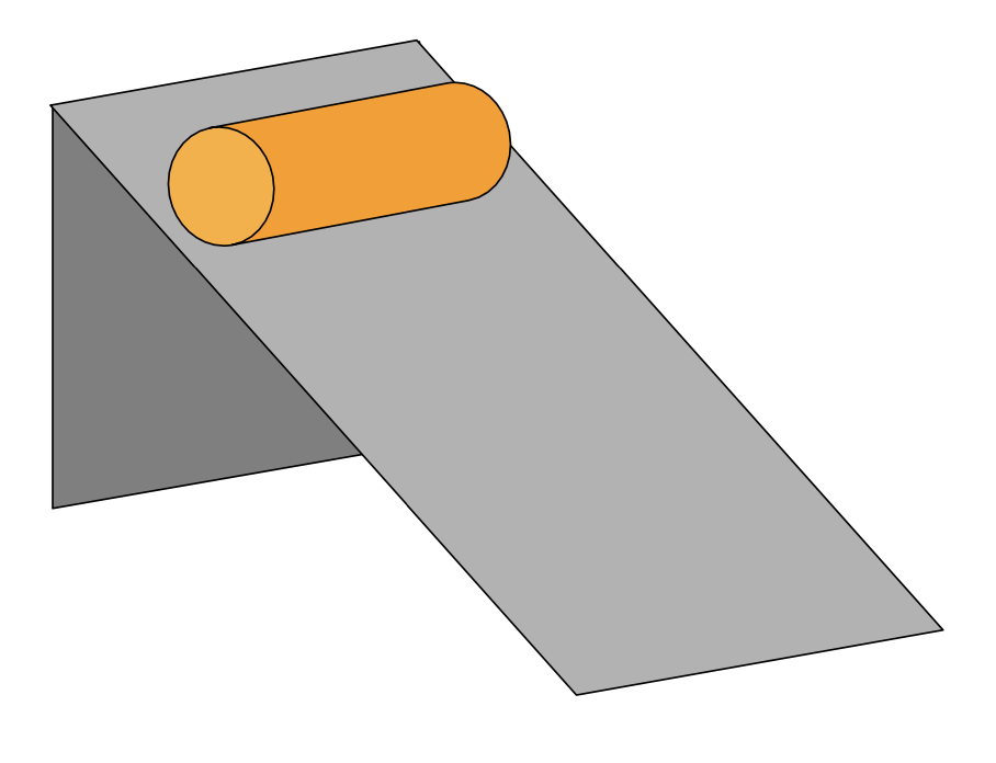
Given a cylinder of radius and mass rolling on an inclined plane with angle %22%2F%3E%3C%2Fg%3E%3C%2Fg%3E%3Cdefs%3E%3Csymbol%20id%3D%22a%22%20overflow%3D%22visible%22%3E%3Cpath%20d%3D%22M4.65%206.63c-1.035%200-1.965-.45-2.79-1.335S.615%203.435.615%202.385c0-1.47.99-2.55%202.46-2.55%201.035%200%202.055.405%203.075%201.2.225-.795.69-1.2%201.38-1.2.54%200%201.305.57%201.305%201.11%200%20.135-.075.195-.24.195-.105%200-.195-.06-.24-.18-.12-.315-.435-.69-.78-.69-.255%200-.39.48-.39%201.455%200%20.21.045.375.135.48A7.7%207.7%200%200%201%208.37%203.9c.375.81.6%201.41.66%201.8v.06c-.045.105-.135.15-.24.15-.075-.015-.165-.135-.27-.345-.315-1.08-.75-2.01-1.335-2.775v.75c0%201.74-.87%203.09-2.535%203.09m1.395-3.465c0-.885.015-1.425.03-1.62C5.1.69%204.11.27%203.105.27%202.25.27%201.83.795%201.83%201.83c0%20.87.495%202.49.84%203.03.57.885%201.23%201.335%201.965%201.335.465%200%20.78-.18.975-.54.105-.18.18-.36.255-.525.12-.345.18-1.26.18-1.965%22%2F%3E%3C%2Fsymbol%3E%3C%2Fdefs%3E%3C%2Fsvg%3E) ,
the question can be simplified by considering the following system:
,
the question can be simplified by considering the following system:
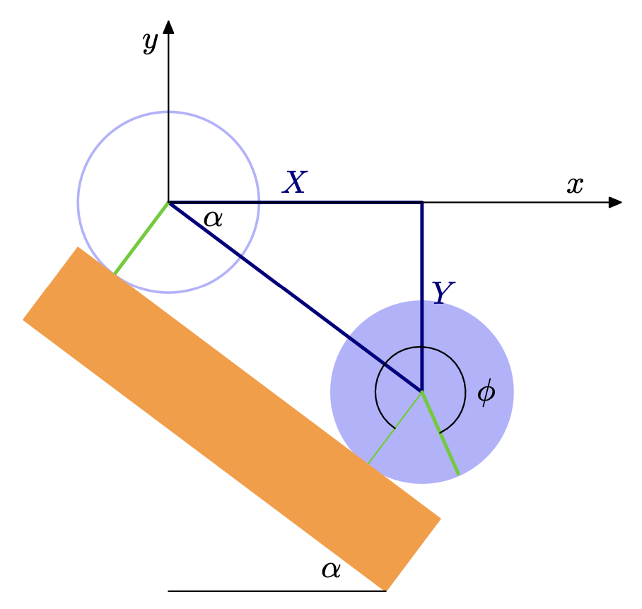
Where is again the angle of the inclined plane,
%22%2F%3E%3C%2Fg%3E%3C%2Fg%3E%3Cdefs%3E%3Csymbol%20id%3D%22a%22%20overflow%3D%22visible%22%3E%3Cpath%20d%3D%22M5.775%206.675c.285%201.185.585%202.34.855%203.525v.045c-.045.105-.12.165-.24.165-.135%200-.225-.12-.27-.345l-.855-3.39C4.14%206.63%203.12%206.21%202.205%205.43%201.23%204.605.735%203.645.735%202.55.735.93%201.98-.105%203.555-.195c-.285-1.185-.495-2.04-.63-2.55-.015-.045-.015-.09-.015-.105%200-.15.075-.225.24-.225s.21.09.255.27l.66%202.595c1.125.045%202.145.465%203.06%201.245.975.84%201.47%201.8%201.47%202.895%200%201.605-1.275%202.61-2.82%202.745m-.12-.45c1.14-.075%201.86-.78%201.86-1.98%200-.6-.135-1.2-.405-1.785C6.63%201.38%205.535.39%204.17.255Zm-3.84-3.99c0%20.6.135%201.2.405%201.785.48%201.08%201.575%202.055%202.925%202.205L3.66.24c-1.125.09-1.845.795-1.845%201.995%22%2F%3E%3C%2Fsymbol%3E%3C%2Fdefs%3E%3C%2Fsvg%3E) is the rolling angle of the cylinder,
and
is the rolling angle of the cylinder,
and %22%2F%3E%3Cuse%20xlink%3Ahref%3D%22%23b%22%20class%3D%22typst-text%22%20transform%3D%22matrix(1%200%200%20-1%2016.912%2012.22)%22%2F%3E%3Cuse%20xlink%3Ahref%3D%22%23c%22%20class%3D%22typst-text%22%20transform%3D%22matrix(1%200%200%20-1%2032.748%2012.22)%22%2F%3E%3Cuse%20xlink%3Ahref%3D%22%23d%22%20class%3D%22typst-text%22%20transform%3D%22matrix(1%200%200%20-1%2038.583%2012.22)%22%2F%3E%3Cuse%20xlink%3Ahref%3D%22%23e%22%20class%3D%22typst-text%22%20transform%3D%22matrix(1%200%200%20-1%2047.163%2012.22)%22%2F%3E%3Cuse%20xlink%3Ahref%3D%22%23f%22%20class%3D%22typst-text%22%20transform%3D%22matrix(1%200%200%20-1%2053.833%2012.22)%22%2F%3E%3Cuse%20xlink%3Ahref%3D%22%23g%22%20class%3D%22typst-text%22%20transform%3D%22matrix(1%200%200%20-1%2061.603%2012.22)%22%2F%3E%3C%2Fg%3E%3C%2Fg%3E%3Cdefs%3E%3Csymbol%20id%3D%22a%22%20overflow%3D%22visible%22%3E%3Cpath%20d%3D%22M11.085%207.965c0%20.765-.39%201.35-1.155%201.77-.615.345-1.35.51-2.175.51h-4.23c-.345%200-.495-.015-.495-.36%200-.105.045-.18.135-.195.15-.015.27-.03.345-.03.45-.015.705-.045.78-.06s.12-.06.12-.135c0-.03-.015-.12-.06-.27L2.37%201.23C2.295.9%202.145.69%201.92.615%201.815.585%201.545.57%201.08.57.75.57.615.555.615.225q0-.247.27-.225l1.86.045L4.635%200c.24-.015.36.12.36.345%200%20.15-.165.225-.48.225-.6%200-.9.075-.9.21%200%200%20.015.03.045.24l.96%203.885h1.725c1.035%200%201.56-.435%201.56-1.29%200-.135-.075-.465-.21-1.005-.165-.63-.24-1.05-.24-1.275C7.455.195%208.34-.33%209.48-.33c.42%200%20.825.195%201.23.57s.615.78.615%201.2c0%20.15-.075.225-.24.225-.105%200-.195-.075-.24-.24C10.68.96%2010.47.615%2010.23.42s-.465-.3-.69-.3c-.345%200-.525.285-.525.84%200%20.36.045.915.15%201.68.045.315.06.54.06.705%200%20.795-.42%201.38-1.26%201.74%201.41.345%203.12%201.35%203.12%202.88M9.135%209.24q.45-.293.45-.99c0-.3-.06-.645-.195-1.05q-.607-1.845-3.06-1.845H4.74l.945%203.795q.113.472.36.495c.075.015.375.015.9.015.975%200%201.545-.03%202.19-.42%22%2F%3E%3C%2Fsymbol%3E%3Csymbol%20id%3D%22b%22%20overflow%3D%22visible%22%3E%3Cpath%20d%3D%22M10.47%205.505H1.2c-.24%200-.36-.12-.36-.345s.12-.345.36-.345h9.27c.24%200%20.36.12.36.345%200%20.18-.165.345-.36.345m0-2.82H1.2c-.24%200-.36-.12-.36-.345s.12-.345.36-.345h9.27c.24%200%20.36.12.36.345a.35.35%200%200%201-.36.345%22%2F%3E%3C%2Fsymbol%3E%3Csymbol%20id%3D%22c%22%20overflow%3D%22visible%22%3E%3Cpath%20d%3D%22M4.77-3.72c.135%200%20.21.075.21.21%200%20.045-.03.105-.075.165-.78.6-1.41%201.59-1.875%202.955-.405%201.185-.615%202.355-.615%203.51v1.26c0%201.155.21%202.325.615%203.51.465%201.365%201.095%202.355%201.875%202.955a.24.24%200%200%201%20.075.165c0%20.135-.075.21-.21.21a.3.3%200%200%201-.105-.045c-.9-.69-1.65-1.71-2.265-3.075-.585-1.305-.885-2.535-.885-3.72V3.12c0-1.185.3-2.415.885-3.72.615-1.365%201.365-2.385%202.265-3.075a.3.3%200%200%201%20.105-.045%22%2F%3E%3C%2Fsymbol%3E%3Csymbol%20id%3D%22d%22%20overflow%3D%22visible%22%3E%3Cpath%20d%3D%22M7.905%205.595c0%20.69-.675%201.035-1.425%201.035-.645%200-1.155-.345-1.545-1.035-.315.69-.84%201.035-1.605%201.035-.735%200-1.335-.345-1.815-1.02C1.11%205.025.9%204.59.9%204.305c0-.135.075-.21.225-.21.135%200%20.225.075.255.21.285.87.915%201.89%201.92%201.89.495%200%20.735-.315.735-.93%200-.315-.27-1.485-.795-3.495C2.985.765%202.535.27%201.89.27c-.21%200-.405.045-.57.12q.585.225.585.81c0%20.39-.195.585-.6.585-.495%200-.87-.42-.87-.915%200-.69.705-1.035%201.44-1.035.63%200%201.14.345%201.545%201.035.285-.69.825-1.035%201.605-1.035.72%200%201.32.345%201.8%201.02.405.585.615%201.02.615%201.305%200%20.135-.075.21-.225.21-.135%200-.21-.075-.255-.21C6.705%201.305%206.03.27%205.055.27c-.495%200-.75.3-.75.915%200%20.195.075.615.24%201.29l.51%202.025c.285%201.125.75%201.695%201.41%201.695.21%200%20.405-.045.57-.12-.405-.135-.6-.405-.6-.81%200-.39.21-.585.615-.585.48%200%20.855.435.855.915%22%2F%3E%3C%2Fsymbol%3E%3Csymbol%20id%3D%22e%22%20overflow%3D%22visible%22%3E%3Cpath%20d%3D%22M2.085%201.59c-.48%200-.795-.36-.795-.84%200-.45.345-.825.795-.825.21%200%20.39.06.525.195L2.625%200c0-.945-.315-1.755-.945-2.4-.105-.12-.165-.21-.165-.27%200-.15.06-.225.195-.225s.315.18.57.525c.51.72.765%201.515.765%202.37%200%20.795-.27%201.59-.96%201.59%22%2F%3E%3C%2Fsymbol%3E%3Csymbol%20id%3D%22f%22%20overflow%3D%22visible%22%3E%3Cpath%20d%3D%22M2.445%206.63Q1.432%206.63.87%205.505C.585%204.92.435%204.515.435%204.29c0-.135.075-.21.24-.21.21%200%20.225.09.285.315.345%201.185.825%201.785%201.44%201.785.195%200%20.3-.135.3-.405%200-.24-.075-.585-.24-1.02-.57-1.545-.855-2.58-.855-3.135%200-1.14.705-1.815%201.86-1.815.495%200%20.96.18%201.38.54q-.788-2.97-2.475-2.97-.765%200-1.035.495.9.045.9.855c0%20.375-.195.57-.6.57-.555%200-.885-.465-.885-1.02%200-.825.75-1.35%201.62-1.35%201.725%200%203.135%201.59%203.51%203.06l1.41%205.67c.045.165.06.285.06.36%200%20.3-.165.45-.48.45-.24%200-.435-.12-.57-.345-.09-.315-.165-.585-.21-.81l-.96-3.855C4.98.915%204.185.24%203.51.24c-.57%200-.855.375-.855%201.14%200%20.63.255%201.59.75%202.88.195.525.3.885.3%201.095%200%20.735-.525%201.275-1.26%201.275%22%2F%3E%3C%2Fsymbol%3E%3Csymbol%20id%3D%22g%22%20overflow%3D%22visible%22%3E%3Cpath%20d%3D%22M1.17-3.675c.9.69%201.65%201.71%202.265%203.075.585%201.305.885%202.535.885%203.72v1.26c0%201.185-.3%202.415-.885%203.72-.615%201.365-1.365%202.385-2.265%203.075a.3.3%200%200%201-.105.045c-.135%200-.21-.075-.21-.21%200-.06.03-.12.075-.165.78-.6%201.41-1.59%201.875-2.955.405-1.185.615-2.355.615-3.51V3.12c0-1.155-.21-2.325-.615-3.51C2.34-1.755%201.71-2.745.93-3.345c-.045-.06-.075-.12-.075-.165%200-.135.075-.21.21-.21.015%200%20.06.015.105.045%22%2F%3E%3C%2Fsymbol%3E%3C%2Fdefs%3E%3C%2Fsvg%3E) is the position of the center of mass of the cylinder.
is the position of the center of mass of the cylinder.
As the cylinder is rolling on the plane with no sliding, we can formulate the constraints as:

Thus, the velocity of the center of mass of the cylinder is given by:

And the kinetic energy of the cylinder is given by:

If we consider a constant gravitational field acting on the cylinder,
the potential energy of the cylinder is given by:

The Lagrangian of the cylinder is given by:

Using the Euler-Lagrange equation, we can determine the equation of motion of the cylinder.

0.6 Small Oscillations
0.6.1 Harmonic Oscillator
Given a object with mass , spring constant , and displacement %22%2F%3E%3C%2Fg%3E%3C%2Fg%3E%3Cdefs%3E%3Csymbol%20id%3D%22a%22%20overflow%3D%22visible%22%3E%3Cpath%20d%3D%22M7.905%205.595c0%20.69-.675%201.035-1.425%201.035-.645%200-1.155-.345-1.545-1.035-.315.69-.84%201.035-1.605%201.035-.735%200-1.335-.345-1.815-1.02C1.11%205.025.9%204.59.9%204.305c0-.135.075-.21.225-.21.135%200%20.225.075.255.21.285.87.915%201.89%201.92%201.89.495%200%20.735-.315.735-.93%200-.315-.27-1.485-.795-3.495C2.985.765%202.535.27%201.89.27c-.21%200-.405.045-.57.12q.585.225.585.81c0%20.39-.195.585-.6.585-.495%200-.87-.42-.87-.915%200-.69.705-1.035%201.44-1.035.63%200%201.14.345%201.545%201.035.285-.69.825-1.035%201.605-1.035.72%200%201.32.345%201.8%201.02.405.585.615%201.02.615%201.305%200%20.135-.075.21-.225.21-.135%200-.21-.075-.255-.21C6.705%201.305%206.03.27%205.055.27c-.495%200-.75.3-.75.915%200%20.195.075.615.24%201.29l.51%202.025c.285%201.125.75%201.695%201.41%201.695.21%200%20.405-.045.57-.12-.405-.135-.6-.405-.6-.81%200-.39.21-.585.615-.585.48%200%20.855.435.855.915%22%2F%3E%3C%2Fsymbol%3E%3C%2Fdefs%3E%3C%2Fsvg%3E) .
The kinetic energy of the object is given by:
.
The kinetic energy of the object is given by:
%22%2F%3E%3Cuse%20xlink%3Ahref%3D%22%23b%22%20class%3D%22typst-text%22%20transform%3D%22matrix(1%200%200%20-1%2025.147%2030.145)%22%2F%3E%3Cuse%20xlink%3Ahref%3D%22%23c%22%20class%3D%22typst-text%22%20transform%3D%22matrix(1%200%200%20-1%2042.483%2019.99)%22%2F%3E%3Cuse%20xlink%3Ahref%3D%22%23d%22%20class%3D%22typst-text%22%20transform%3D%22matrix(1%200%200%20-1%2042.483%2040.435)%22%2F%3E%3Cpath%20fill%3D%22none%22%20stroke%3D%22%23000%22%20stroke-width%3D%22.72%22%20d%3D%22M42.483%2026.395h7.5%22%20class%3D%22typst-shape%22%2F%3E%3Cuse%20xlink%3Ahref%3D%22%23e%22%20class%3D%22typst-text%22%20transform%3D%22matrix(1%200%200%20-1%2051.483%2030.145)%22%2F%3E%3Cuse%20xlink%3Ahref%3D%22%23f%22%20class%3D%22typst-text%22%20transform%3D%22matrix(1%200%200%20-1%2073.563%2030.265)%22%2F%3E%3Cuse%20xlink%3Ahref%3D%22%23g%22%20class%3D%22typst-text%22%20transform%3D%22matrix(1%200%200%20-1%2064.653%2030.145)%22%2F%3E%3Cuse%20xlink%3Ahref%3D%22%23h%22%20class%3D%22typst-text%22%20transform%3D%22matrix(1%200%200%20-1%2073.233%2024.7)%22%2F%3E%3C%2Fg%3E%3C%2Fg%3E%3Cdefs%3E%3Csymbol%20id%3D%22a%22%20overflow%3D%22visible%22%3E%3Cpath%20d%3D%22M5.16%209.465c0-.045-.015-.15-.06-.3l-1.98-7.92c-.06-.225-.12-.36-.165-.42C2.82.66%202.31.585%201.41.585.945.585.735.63.735.24c0-.165.105-.24.3-.24.765%200%201.845.06%202.49.045L4.755.03C4.965.03%205.79%200%206.045%200s.375.12.375.36c0%20.15-.18.225-.555.225-.78%200-1.23.03-1.365.105-.045.03-.075.09-.075.18L6.45%209.045c.045.21.09.345.135.39q.09.135%201.08.135c.825%200%201.395-.06%201.68-.195s.435-.45.435-.96c0-.27-.045-.66-.12-1.17-.03-.12-.045-.21-.045-.285%200-.165.075-.255.24-.255.135%200%20.225.135.27.39l.405%202.58c.015.075.03.165.03.255%200%20.15-.15.225-.465.225h-8.22c-.39%200-.42-.045-.54-.33L.45%207.215a5%205%200%200%201-.09-.285c0-.15.075-.225.24-.225.12%200%20.225.12.3.345.375%201.095.75%201.77%201.095%202.055.39.315%201.14.465%202.235.465h.585c.165%200%20.345.015.345-.105%22%2F%3E%3C%2Fsymbol%3E%3Csymbol%20id%3D%22b%22%20overflow%3D%22visible%22%3E%3Cpath%20d%3D%22M10.47%205.505H1.2c-.24%200-.36-.12-.36-.345s.12-.345.36-.345h9.27c.24%200%20.36.12.36.345%200%20.18-.165.345-.36.345m0-2.82H1.2c-.24%200-.36-.12-.36-.345s.12-.345.36-.345h9.27c.24%200%20.36.12.36.345a.35.35%200%200%201-.36.345%22%2F%3E%3C%2Fsymbol%3E%3Csymbol%20id%3D%22c%22%20overflow%3D%22visible%22%3E%3Cpath%20d%3D%22M4.035%209.99q-.922-.945-2.7-.945V8.46c.78%200%201.425.12%201.92.36V1.23c0-.27-.06-.45-.195-.525s-.51-.12-1.11-.12h-.525V0q.563.045%202.43.045T6.285%200v.585H5.76c-.615%200-.99.045-1.11.12s-.195.255-.195.525v8.31c0%20.36-.03.45-.42.45%22%2F%3E%3C%2Fsymbol%3E%3Csymbol%20id%3D%22d%22%20overflow%3D%22visible%22%3E%3Cpath%20d%3D%22M3.555%209.99c-.765%200-1.41-.27-1.965-.81S.75%208.01.75%207.245c0-.51.375-.885.84-.885.45%200%20.825.39.825.84%200%20.495-.36.84-.84.84-.045%200-.075%200-.105-.015.285.735.945%201.38%201.89%201.38%201.23%200%201.92-1.065%201.92-2.355%200-1.005-.51-2.085-1.53-3.225L.93.645C.735.42.75.435.75%200h5.565l.435%202.7h-.495c-.12-.765-.225-1.2-.315-1.335-.075-.075-.525-.105-1.35-.105H2.085L3.54%202.685c1.02.96%202.31%201.995%202.745%202.79q.45.787.45%201.575c0%201.77-1.38%202.94-3.18%202.94%22%2F%3E%3C%2Fsymbol%3E%3Csymbol%20id%3D%22e%22%20overflow%3D%22visible%22%3E%3Cpath%20d%3D%22M9.855%206.63c-.915%200-1.71-.45-2.385-1.335-.135.885-.705%201.335-1.725%201.335-.885%200-1.65-.39-2.28-1.185-.12.66-.645%201.185-1.41%201.185-.615%200-1.065-.495-1.38-1.47-.165-.48-.24-.765-.24-.855%200-.135.075-.21.24-.21a.27.27%200%200%201%20.165.045c.075.135.12.24.15.345.27%201.14.615%201.71%201.02%201.71q.405%200%20.405-.63c0-.195-.075-.6-.24-1.215L1.32.945c-.06-.18-.135-.57-.135-.66%200-.3.165-.45.48-.45.3%200%20.51.15.615.45.015.075.12.45.285%201.095l.315%201.335.45%201.71c.165.345.42.69.75%201.05q.652.72%201.62.72c.495%200%20.735-.33.735-.975q0-.292-.225-1.215l-.405-1.71C5.7%201.86%205.46.96%205.34.48%205.325.375%205.31.315%205.31.285q0-.45.495-.45c.165%200%20.285.045.39.15.225.225.24.33.33.735l.885%203.555c.045.195.255.54.615%201.02.45.6%201.05.9%201.785.9.495%200%20.735-.33.735-.975%200-.585-.3-1.68-.915-3.285-.135-.345-.195-.63-.195-.825%200-.735.555-1.275%201.275-1.275.675%200%201.185.375%201.56%201.125.3.6.45%201.005.45%201.2%200%20.135-.075.21-.24.21-.105-.015-.21-.15-.285-.315C11.865.87%2011.385.27%2010.74.27c-.195%200-.3.15-.3.435%200%20.225.09.555.27%201.02.615%201.605.915%202.7.915%203.27%200%201.065-.705%201.635-1.77%201.635%22%2F%3E%3C%2Fsymbol%3E%3Csymbol%20id%3D%22f%22%20overflow%3D%22visible%22%3E%3Cpath%20d%3D%22M-3.165%209.36a.8.8%200%200%201-.795.795.813.813%200%200%201-.81-.795.8.8%200%200%201%20.795-.795c.435%200%20.81.36.81.795%22%2F%3E%3C%2Fsymbol%3E%3Csymbol%20id%3D%22g%22%20overflow%3D%22visible%22%3E%3Cpath%20d%3D%22M7.905%205.595c0%20.69-.675%201.035-1.425%201.035-.645%200-1.155-.345-1.545-1.035-.315.69-.84%201.035-1.605%201.035-.735%200-1.335-.345-1.815-1.02C1.11%205.025.9%204.59.9%204.305c0-.135.075-.21.225-.21.135%200%20.225.075.255.21.285.87.915%201.89%201.92%201.89.495%200%20.735-.315.735-.93%200-.315-.27-1.485-.795-3.495C2.985.765%202.535.27%201.89.27c-.21%200-.405.045-.57.12q.585.225.585.81c0%20.39-.195.585-.6.585-.495%200-.87-.42-.87-.915%200-.69.705-1.035%201.44-1.035.63%200%201.14.345%201.545%201.035.285-.69.825-1.035%201.605-1.035.72%200%201.32.345%201.8%201.02.405.585.615%201.02.615%201.305%200%20.135-.075.21-.225.21-.135%200-.21-.075-.255-.21C6.705%201.305%206.03.27%205.055.27c-.495%200-.75.3-.75.915%200%20.195.075.615.24%201.29l.51%202.025c.285%201.125.75%201.695%201.41%201.695.21%200%20.405-.045.57-.12-.405-.135-.6-.405-.6-.81%200-.39.21-.585.615-.585.48%200%20.855.435.855.915%22%2F%3E%3C%2Fsymbol%3E%3Csymbol%20id%3D%22h%22%20overflow%3D%22visible%22%3E%3Cpath%20d%3D%22M1.25%204.452c.335%200%20.587.252.587.588%200%20.378-.199.577-.587.588.23.494.756.892%201.438.892.924%200%201.533-.692%201.533-1.616%200-.505-.178-.988-.546-1.46a5%205%200%200%200-.41-.504L.777.473C.64.347.661.315.661%200h4.326l.326%201.974h-.441c-.074-.556-.157-.882-.252-.955-.053-.032-.378-.053-.997-.053H1.837c.704.62%201.355%201.176%201.974%201.67.473.367.809.692%201.019.976q.473.614.473%201.292c0%20.65-.252%201.165-.767%201.543-.451.346-1.018.525-1.69.525a2.36%202.36%200%200%201-1.502-.504c-.452-.367-.683-.83-.683-1.396%200-.357.263-.62.589-.62%22%2F%3E%3C%2Fsymbol%3E%3C%2Fdefs%3E%3C%2Fsvg%3E)
The potential energy of the object is given by:
%22%2F%3E%3Cuse%20xlink%3Ahref%3D%22%23b%22%20class%3D%22typst-text%22%20transform%3D%22matrix(1%200%200%20-1%2025.987%2030.145)%22%2F%3E%3Cuse%20xlink%3Ahref%3D%22%23c%22%20class%3D%22typst-text%22%20transform%3D%22matrix(1%200%200%20-1%2043.323%2019.99)%22%2F%3E%3Cuse%20xlink%3Ahref%3D%22%23d%22%20class%3D%22typst-text%22%20transform%3D%22matrix(1%200%200%20-1%2043.323%2040.435)%22%2F%3E%3Cpath%20fill%3D%22none%22%20stroke%3D%22%23000%22%20stroke-width%3D%22.72%22%20d%3D%22M43.323%2026.395h7.5%22%20class%3D%22typst-shape%22%2F%3E%3Cuse%20xlink%3Ahref%3D%22%23e%22%20class%3D%22typst-text%22%20transform%3D%22matrix(1%200%200%20-1%2052.323%2030.145)%22%2F%3E%3Cuse%20xlink%3Ahref%3D%22%23f%22%20class%3D%22typst-text%22%20transform%3D%22matrix(1%200%200%20-1%2060.363%2030.145)%22%2F%3E%3Cuse%20xlink%3Ahref%3D%22%23g%22%20class%3D%22typst-text%22%20transform%3D%22matrix(1%200%200%20-1%2068.943%2024.7)%22%2F%3E%3C%2Fg%3E%3C%2Fg%3E%3Cdefs%3E%3Csymbol%20id%3D%22a%22%20overflow%3D%22visible%22%3E%3Cpath%20d%3D%22M9.63%2010.2c-.285%200-1.245.045-1.53.045-.225%200-.33-.12-.33-.36q0-.202.315-.225c.645%200%20.96-.195.96-.585%200-.09-.015-.195-.045-.3L7.665%203.48A4.73%204.73%200%200%200%206.36%201.26C5.655.585%204.875.255%204.035.255c-1.11%200-1.755.75-1.755%201.86l.015.135c0%20.285.045.615.15%201.005l1.44%205.775q.112.472.405.585c.09.03.345.045.78.045.39%200%20.555%200%20.555.36%200%20.15-.09.225-.255.225L3.465%2010.2l-1.905.045c-.24%200-.345-.135-.345-.36%200-.105.045-.18.12-.195.15-.015.27-.03.345-.03.465-.015.735-.045.81-.06s.105-.06.105-.135c0-.03-.015-.135-.06-.3L1.11%203.45a3.4%203.4%200%200%201-.105-.87c0-1.725%201.245-2.91%202.97-2.91.975%200%201.875.375%202.7%201.14.795.72%201.305%201.56%201.545%202.535L9.54%208.61c.195.765.615%201.035%201.545%201.05q.315.023.315.36v.06c-.045.105-.12.165-.255.165-.285%200-1.23-.045-1.515-.045%22%2F%3E%3C%2Fsymbol%3E%3Csymbol%20id%3D%22b%22%20overflow%3D%22visible%22%3E%3Cpath%20d%3D%22M10.47%205.505H1.2c-.24%200-.36-.12-.36-.345s.12-.345.36-.345h9.27c.24%200%20.36.12.36.345%200%20.18-.165.345-.36.345m0-2.82H1.2c-.24%200-.36-.12-.36-.345s.12-.345.36-.345h9.27c.24%200%20.36.12.36.345a.35.35%200%200%201-.36.345%22%2F%3E%3C%2Fsymbol%3E%3Csymbol%20id%3D%22c%22%20overflow%3D%22visible%22%3E%3Cpath%20d%3D%22M4.035%209.99q-.922-.945-2.7-.945V8.46c.78%200%201.425.12%201.92.36V1.23c0-.27-.06-.45-.195-.525s-.51-.12-1.11-.12h-.525V0q.563.045%202.43.045T6.285%200v.585H5.76c-.615%200-.99.045-1.11.12s-.195.255-.195.525v8.31c0%20.36-.03.45-.42.45%22%2F%3E%3C%2Fsymbol%3E%3Csymbol%20id%3D%22d%22%20overflow%3D%22visible%22%3E%3Cpath%20d%3D%22M3.555%209.99c-.765%200-1.41-.27-1.965-.81S.75%208.01.75%207.245c0-.51.375-.885.84-.885.45%200%20.825.39.825.84%200%20.495-.36.84-.84.84-.045%200-.075%200-.105-.015.285.735.945%201.38%201.89%201.38%201.23%200%201.92-1.065%201.92-2.355%200-1.005-.51-2.085-1.53-3.225L.93.645C.735.42.75.435.75%200h5.565l.435%202.7h-.495c-.12-.765-.225-1.2-.315-1.335-.075-.075-.525-.105-1.35-.105H2.085L3.54%202.685c1.02.96%202.31%201.995%202.745%202.79q.45.787.45%201.575c0%201.77-1.38%202.94-3.18%202.94%22%2F%3E%3C%2Fsymbol%3E%3Csymbol%20id%3D%22e%22%20overflow%3D%22visible%22%3E%3Cpath%20d%3D%22M6.135%205.295c0-.39.21-.585.615-.585.525%200%20.87.465.87.975%200%20.585-.48.99-1.065.99-.675%200-1.395-.45-2.19-1.335-.615-.675-1.11-1.11-1.515-1.305l1.515%206.15c-.03.135-.06.225-.255.225-.48%200-1.62-.135-1.8-.15-.225-.03-.33-.135-.33-.36q0-.225.405-.225c.285%200%20.675.015.675-.195L.885.645a1.4%201.4%200%200%201-.06-.33c0-.315.165-.48.48-.48.255%200%20.45.12.555.345.075.135.345%201.2.825%203.21.78-.075%201.605-.45%201.605-1.2%200-.225-.105-.675-.105-.825%200-.855.555-1.53%201.41-1.53q1.305%200%201.755%202.34c0%20.135-.075.21-.225.21q-.202%200-.27-.315C6.525.885%206.12.285%205.625.285q-.405%200-.405.63c0%20.24.18%201.05.18%201.29%200%20.855-.69%201.38-2.085%201.59.345.24.735.585%201.155%201.035s.72.735.915.9c.405.33.795.495%201.14.495q.225%200%20.36-.09c-.405-.075-.75-.45-.75-.84%22%2F%3E%3C%2Fsymbol%3E%3Csymbol%20id%3D%22f%22%20overflow%3D%22visible%22%3E%3Cpath%20d%3D%22M7.905%205.595c0%20.69-.675%201.035-1.425%201.035-.645%200-1.155-.345-1.545-1.035-.315.69-.84%201.035-1.605%201.035-.735%200-1.335-.345-1.815-1.02C1.11%205.025.9%204.59.9%204.305c0-.135.075-.21.225-.21.135%200%20.225.075.255.21.285.87.915%201.89%201.92%201.89.495%200%20.735-.315.735-.93%200-.315-.27-1.485-.795-3.495C2.985.765%202.535.27%201.89.27c-.21%200-.405.045-.57.12q.585.225.585.81c0%20.39-.195.585-.6.585-.495%200-.87-.42-.87-.915%200-.69.705-1.035%201.44-1.035.63%200%201.14.345%201.545%201.035.285-.69.825-1.035%201.605-1.035.72%200%201.32.345%201.8%201.02.405.585.615%201.02.615%201.305%200%20.135-.075.21-.225.21-.135%200-.21-.075-.255-.21C6.705%201.305%206.03.27%205.055.27c-.495%200-.75.3-.75.915%200%20.195.075.615.24%201.29l.51%202.025c.285%201.125.75%201.695%201.41%201.695.21%200%20.405-.045.57-.12-.405-.135-.6-.405-.6-.81%200-.39.21-.585.615-.585.48%200%20.855.435.855.915%22%2F%3E%3C%2Fsymbol%3E%3Csymbol%20id%3D%22g%22%20overflow%3D%22visible%22%3E%3Cpath%20d%3D%22M1.25%204.452c.335%200%20.587.252.587.588%200%20.378-.199.577-.587.588.23.494.756.892%201.438.892.924%200%201.533-.692%201.533-1.616%200-.505-.178-.988-.546-1.46a5%205%200%200%200-.41-.504L.777.473C.64.347.661.315.661%200h4.326l.326%201.974h-.441c-.074-.556-.157-.882-.252-.955-.053-.032-.378-.053-.997-.053H1.837c.704.62%201.355%201.176%201.974%201.67.473.367.809.692%201.019.976q.473.614.473%201.292c0%20.65-.252%201.165-.767%201.543-.451.346-1.018.525-1.69.525a2.36%202.36%200%200%201-1.502-.504c-.452-.367-.683-.83-.683-1.396%200-.357.263-.62.589-.62%22%2F%3E%3C%2Fsymbol%3E%3C%2Fdefs%3E%3C%2Fsvg%3E)
The Lagrangian of the object is given by:

By solving the Euler-Lagrange equation, we can determine the equation of motion of the object.

Thus,

0.6.2 Small Oscillations in General
Given a system with generalized coordinates ,
and potential energy of the system.
And stationary points %22%2F%3E%3Cuse%20xlink%3Ahref%3D%22%23b%22%20class%3D%22typst-text%22%20transform%3D%22matrix(1%200%200%20-1%207.69%2011.335)%22%2F%3E%3Cuse%20xlink%3Ahref%3D%22%23c%22%20class%3D%22typst-text%22%20transform%3D%22matrix(1%200%200%20-1%2011.932%2011.335)%22%2F%3E%3C%2Fg%3E%3C%2Fg%3E%3Cdefs%3E%3Csymbol%20id%3D%22a%22%20overflow%3D%22visible%22%3E%3Cpath%20d%3D%22M5.58%205.655c-.3.645-.765.975-1.38.975-.975%200-1.83-.495-2.565-1.5C.945%204.2.6%203.24.6%202.235c0-1.305.75-2.43%201.995-2.43.54%200%201.08.255%201.635.765l-.615-2.46a.48.48%200%200%200-.39-.405%204%204%200%200%200-.615-.03c-.09-.015-.15-.015-.18-.015-.135-.015-.21-.135-.21-.345v-.06a.26.26%200%200%201%20.255-.165c.285%200%201.185.045%201.47.045s1.23-.045%201.515-.045q.315%200%20.315.36c0%20.15-.15.225-.435.225-.27%200-.645-.015-.645.165%200%20.06.015.165.06.315l2.025%208.25c0%20.135-.075.21-.21.21-.27%200-.84-.75-.99-.96m-.48-.06c.135-.315.21-.525.21-.66a2%202%200%200%200-.045-.24l-.36-1.455c-.285-1.08-.42-1.635-.435-1.665C4.185%201.05%203.36.24%202.64.24c-.585%200-.885.45-.885%201.335%200%20.69.465%202.37.675%202.925.285.705.945%201.68%201.77%201.68q.607%200%20.9-.585%22%2F%3E%3C%2Fsymbol%3E%3Csymbol%20id%3D%22b%22%20overflow%3D%22visible%22%3E%3Cpath%20d%3D%22M3.413%206.52a.44.44%200%200%201-.452.441c-.315%200-.62-.293-.62-.609%200-.252.2-.44.452-.44.315%200%20.62.293.62.608M2.016%204.662q-.74%200-1.165-.756c-.242-.42-.357-.714-.357-.882%200-.115.073-.168.21-.168q.17%200%20.23.189c.242.83.588%201.239%201.05%201.239.147%200%20.221-.105.221-.325%200-.137-.105-.473-.315-1.019l-.651-1.67a1.3%201.3%200%200%201-.095-.45c0-.546.473-.924%201.019-.924.493%200%20.872.252%201.155.767.241.42.357.703.357.86%200%20.116-.073.179-.21.179-.063-.01-.136-.063-.21-.168a.1.1%200%200%201-.021-.042C2.993.682%202.646.273%202.194.273q-.22%200-.22.315c0%20.157.052.378.168.651l.83%202.153q.063.172.063.346c0%20.546-.473.924-1.019.924%22%2F%3E%3C%2Fsymbol%3E%3Csymbol%20id%3D%22c%22%20overflow%3D%22visible%22%3E%3Cpath%20d%3D%22M5.418%203.35c0%201.186-.21%202.089-.62%202.709-.335.524-1.007.913-1.816.913-.336%200-.64-.053-.903-.168C.924%206.321.546%204.977.546%203.349c0-.357.021-.693.052-1.018C.778.956%201.418-.21%202.983-.21c.336%200%20.64.052.903.168C5.04.431%205.418%201.743%205.418%203.349M4.221%205.68c.115-.388.178-1.112.178-2.194%200-1.029-.042-1.754-.136-2.184C4.137.682%203.696.168%202.982.168c-.263%200-.525.084-.767.262-.325.242-.524.715-.608%201.439-.032.241-.042.777-.042%201.617%200%201.019.052%201.722.157%202.1q.268%201.008%201.26%201.008c.63%200%201.092-.41%201.239-.913%22%2F%3E%3C%2Fsymbol%3E%3C%2Fdefs%3E%3C%2Fsvg%3E) of potential energy .
Such that
of potential energy .
Such that
%22%2F%3E%3Cuse%20xlink%3Ahref%3D%22%23b%22%20class%3D%22typst-text%22%20transform%3D%22matrix(1%200%200%20-1%2020.41%2020.74)%22%2F%3E%3Cuse%20xlink%3Ahref%3D%22%23a%22%20class%3D%22typst-text%22%20transform%3D%22matrix(1%200%200%20-1%2011.524%2041.185)%22%2F%3E%3Cuse%20xlink%3Ahref%3D%22%23c%22%20class%3D%22typst-text%22%20transform%3D%22matrix(1%200%200%20-1%2020.434%2041.185)%22%2F%3E%3Cuse%20xlink%3Ahref%3D%22%23d%22%20class%3D%22typst-text%22%20transform%3D%22matrix(1%200%200%20-1%2027.124%2044.89)%22%2F%3E%3Cpath%20fill%3D%22none%22%20stroke%3D%22%23000%22%20stroke-width%3D%22.72%22%20d%3D%22M11.5%2027.145h20.73%22%20class%3D%22typst-shape%22%2F%3E%3Cuse%20xlink%3Ahref%3D%22%23e%22%20class%3D%22typst-text%22%20transform%3D%22matrix(1%200%200%20-1%2037.897%2030.895)%22%2F%3E%3Cuse%20xlink%3Ahref%3D%22%23f%22%20class%3D%22typst-text%22%20transform%3D%22matrix(1%200%200%20-1%2053.733%2030.895)%22%2F%3E%3C%2Fg%3E%3C%2Fg%3E%3Cdefs%3E%3Csymbol%20id%3D%22a%22%20overflow%3D%22visible%22%3E%3Cpath%20d%3D%22M3.84%208.61c0%20.345-.225.54-.66.57.465.705%201.14%201.065%202.025%201.065%201.38%200%202.055-1.155%202.055-2.625%200-.615-.12-1.365-.345-2.28-.255%201.035-.9%201.56-1.905%201.56-1.155%200-2.16-.48-3.06-1.41S.6%203.525.6%202.37c0-.555.195-1.125.585-1.695C1.65%200%202.37-.33%203.375-.33c1.35%200%202.475.63%203.36%201.905.84%201.23%201.755%203.36%201.755%205.265%200%201.065-.27%201.965-.81%202.685-.585.81-1.41%201.215-2.445%201.215-1.005%200-1.755-.345-2.265-1.05-.405-.555-.615-1.005-.615-1.35q0-.585.63-.585c.45%200%20.855.405.855.855m2.745-4.065c0-.945-.285-1.875-.87-2.79C5.07.72%204.305.21%203.42.21c-.99%200-1.56.645-1.56%201.605q0%20.63.315%201.755c.21.75.42%201.275.645%201.59.6.855%201.335%201.29%202.19%201.29%201.095%200%201.575-.81%201.575-1.905%22%2F%3E%3C%2Fsymbol%3E%3Csymbol%20id%3D%22b%22%20overflow%3D%22visible%22%3E%3Cpath%20d%3D%22M9.63%2010.2c-.285%200-1.245.045-1.53.045-.225%200-.33-.12-.33-.36q0-.202.315-.225c.645%200%20.96-.195.96-.585%200-.09-.015-.195-.045-.3L7.665%203.48A4.73%204.73%200%200%200%206.36%201.26C5.655.585%204.875.255%204.035.255c-1.11%200-1.755.75-1.755%201.86l.015.135c0%20.285.045.615.15%201.005l1.44%205.775q.112.472.405.585c.09.03.345.045.78.045.39%200%20.555%200%20.555.36%200%20.15-.09.225-.255.225L3.465%2010.2l-1.905.045c-.24%200-.345-.135-.345-.36%200-.105.045-.18.12-.195.15-.015.27-.03.345-.03.465-.015.735-.045.81-.06s.105-.06.105-.135c0-.03-.015-.135-.06-.3L1.11%203.45a3.4%203.4%200%200%201-.105-.87c0-1.725%201.245-2.91%202.97-2.91.975%200%201.875.375%202.7%201.14.795.72%201.305%201.56%201.545%202.535L9.54%208.61c.195.765.615%201.035%201.545%201.05q.315.023.315.36v.06c-.045.105-.12.165-.255.165-.285%200-1.23-.045-1.515-.045%22%2F%3E%3C%2Fsymbol%3E%3Csymbol%20id%3D%22c%22%20overflow%3D%22visible%22%3E%3Cpath%20d%3D%22M5.58%205.655c-.3.645-.765.975-1.38.975-.975%200-1.83-.495-2.565-1.5C.945%204.2.6%203.24.6%202.235c0-1.305.75-2.43%201.995-2.43.54%200%201.08.255%201.635.765l-.615-2.46a.48.48%200%200%200-.39-.405%204%204%200%200%200-.615-.03c-.09-.015-.15-.015-.18-.015-.135-.015-.21-.135-.21-.345v-.06a.26.26%200%200%201%20.255-.165c.285%200%201.185.045%201.47.045s1.23-.045%201.515-.045q.315%200%20.315.36c0%20.15-.15.225-.435.225-.27%200-.645-.015-.645.165%200%20.06.015.165.06.315l2.025%208.25c0%20.135-.075.21-.21.21-.27%200-.84-.75-.99-.96m-.48-.06c.135-.315.21-.525.21-.66a2%202%200%200%200-.045-.24l-.36-1.455c-.285-1.08-.42-1.635-.435-1.665C4.185%201.05%203.36.24%202.64.24c-.585%200-.885.45-.885%201.335%200%20.69.465%202.37.675%202.925.285.705.945%201.68%201.77%201.68q.607%200%20.9-.585%22%2F%3E%3C%2Fsymbol%3E%3Csymbol%20id%3D%22d%22%20overflow%3D%22visible%22%3E%3Cpath%20d%3D%22M3.413%206.52a.44.44%200%200%201-.452.441c-.315%200-.62-.293-.62-.609%200-.252.2-.44.452-.44.315%200%20.62.293.62.608M2.016%204.662q-.74%200-1.165-.756c-.242-.42-.357-.714-.357-.882%200-.115.073-.168.21-.168q.17%200%20.23.189c.242.83.588%201.239%201.05%201.239.147%200%20.221-.105.221-.325%200-.137-.105-.473-.315-1.019l-.651-1.67a1.3%201.3%200%200%201-.095-.45c0-.546.473-.924%201.019-.924.493%200%20.872.252%201.155.767.241.42.357.703.357.86%200%20.116-.073.179-.21.179-.063-.01-.136-.063-.21-.168a.1.1%200%200%201-.021-.042C2.993.682%202.646.273%202.194.273q-.22%200-.22.315c0%20.157.052.378.168.651l.83%202.153q.063.172.063.346c0%20.546-.473.924-1.019.924%22%2F%3E%3C%2Fsymbol%3E%3Csymbol%20id%3D%22e%22%20overflow%3D%22visible%22%3E%3Cpath%20d%3D%22M10.47%205.505H1.2c-.24%200-.36-.12-.36-.345s.12-.345.36-.345h9.27c.24%200%20.36.12.36.345%200%20.18-.165.345-.36.345m0-2.82H1.2c-.24%200-.36-.12-.36-.345s.12-.345.36-.345h9.27c.24%200%20.36.12.36.345a.35.35%200%200%201-.36.345%22%2F%3E%3C%2Fsymbol%3E%3Csymbol%20id%3D%22f%22%20overflow%3D%22visible%22%3E%3Cpath%20d%3D%22M3.735-.33C5.85-.33%206.9%201.38%206.9%204.8c0%202.295-.48%203.825-1.425%204.575-.525.405-1.11.615-1.725.615C1.635%209.99.585%208.265.585%204.8c0-2.76.735-5.13%203.15-5.13m1.68%208.19c.105-.525.15-1.485.15-2.88%200-1.38-.06-2.4-.165-3.06Q5.107.12%203.735.12c-.345%200-.69.135-1.005.39-.405.345-.645%201.05-.75%202.13-.045.375-.06%201.155-.06%202.34%200%201.305.045%202.22.12%202.715.135.825.405%201.35.825%201.575.33.18.615.27.87.27.975%200%201.515-.795%201.68-1.68%22%2F%3E%3C%2Fsymbol%3E%3C%2Fdefs%3E%3C%2Fsvg%3E)
Then, the potential energy can be expanded as a Taylor series around the stationary points .

We could use symmetric matrix %22%2F%3E%3C%2Fg%3E%3C%2Fg%3E%3Cdefs%3E%3Csymbol%20id%3D%22a%22%20overflow%3D%22visible%22%3E%3Cpath%20d%3D%22M12.06%2010.2c-.315%200-1.335.045-1.65.045-.225%200-.345-.12-.345-.36%200-.12.105-.195.315-.24s.33-.12.33-.225c0-.165-.165-.39-.51-.645L4.53%204.44l1.155%204.59q.113.472.405.585c.09.03.345.045.78.045.39%200%20.57%200%20.57.36q0%20.225-.27.225L5.265%2010.2l-1.92.045c-.24.015-.36-.105-.36-.345%200-.165.165-.24.495-.24.3%200%20.915.045.915-.195%200-.03-.015-.12-.06-.27L2.34%201.23C2.265.9%202.115.705%201.89.63%201.785.6%201.515.585%201.05.585.72.585.57.555.57.24.57.075.66%200%20.855%200l1.89.045L3.69.03c.165%200%20.795-.03.96-.03q.36%200%20.36.36c0%20.15-.15.225-.465.225-.615%200-.915.06-.915.195%200%20.075.045.3.135.645l.585%202.31%202.145%201.65L8.19%201.47c.105-.255.165-.42.165-.495%200-.255-.24-.39-.705-.39-.27%200-.39-.06-.39-.36Q7.26%200%207.53%200c.33%200%201.47.045%201.8.045C9.615.045%2010.515%200%2010.8%200q.315%200%20.315.36c0%20.135-.12.21-.345.225-.615%200-.765.165-.975.63L7.68%206.06c-.015.075-.045.135-.06.18l3%202.31c.735.57%201.365.915%201.875%201.035.36.06.84.045.84.435q0%20.225-.225.225c-.21%200-.84-.045-1.05-.045%22%2F%3E%3C%2Fsymbol%3E%3C%2Fdefs%3E%3C%2Fsvg%3E) to represent the second order partial derivatives of the potential energy .
to represent the second order partial derivatives of the potential energy .
%22%2F%3E%3Cuse%20xlink%3Ahref%3D%22%23b%22%20class%3D%22typst-text%22%20transform%3D%22matrix(1%200%200%20-1%2022.285%2036.277)%22%2F%3E%3Cuse%20xlink%3Ahref%3D%22%23c%22%20class%3D%22typst-text%22%20transform%3D%22matrix(1%200%200%20-1%2026.527%2036.277)%22%2F%3E%3Cuse%20xlink%3Ahref%3D%22%23d%22%20class%3D%22typst-text%22%20transform%3D%22matrix(1%200%200%20-1%2036.5%2032.572)%22%2F%3E%3Cuse%20xlink%3Ahref%3D%22%23e%22%20class%3D%22typst-text%22%20transform%3D%22matrix(1%200%200%20-1%2061.109%2022.417)%22%2F%3E%3Cuse%20xlink%3Ahref%3D%22%23f%22%20class%3D%22typst-text%22%20transform%3D%22matrix(1%200%200%20-1%2070.019%2016.972)%22%2F%3E%3Cuse%20xlink%3Ahref%3D%22%23g%22%20class%3D%22typst-text%22%20transform%3D%22matrix(1%200%200%20-1%2076.833%2022.417)%22%2F%3E%3Cg%20class%3D%22typst-group%22%3E%3Cuse%20xlink%3Ahref%3D%22%23e%22%20class%3D%22typst-text%22%20transform%3D%22matrix(1%200%200%20-1%2053.837%2042.862)%22%2F%3E%3Cuse%20xlink%3Ahref%3D%22%23h%22%20class%3D%22typst-text%22%20transform%3D%22matrix(1%200%200%20-1%2062.747%2042.862)%22%2F%3E%3Cuse%20xlink%3Ahref%3D%22%23b%22%20class%3D%22typst-text%22%20transform%3D%22matrix(1%200%200%20-1%2069.437%2046.567)%22%2F%3E%3Cuse%20xlink%3Ahref%3D%22%23e%22%20class%3D%22typst-text%22%20transform%3D%22matrix(1%200%200%20-1%2074.519%2042.862)%22%2F%3E%3Cuse%20xlink%3Ahref%3D%22%23h%22%20class%3D%22typst-text%22%20transform%3D%22matrix(1%200%200%20-1%2083.429%2042.862)%22%2F%3E%3Cuse%20xlink%3Ahref%3D%22%23c%22%20class%3D%22typst-text%22%20transform%3D%22matrix(1%200%200%20-1%2090.119%2046.567)%22%2F%3E%3C%2Fg%3E%3Cpath%20fill%3D%22none%22%20stroke%3D%22%23000%22%20stroke-width%3D%22.72%22%20d%3D%22M53.837%2028.822h42.088%22%20class%3D%22typst-shape%22%2F%3E%3C%2Fg%3E%3C%2Fg%3E%3Cdefs%3E%3Csymbol%20id%3D%22a%22%20overflow%3D%22visible%22%3E%3Cpath%20d%3D%22M12.06%2010.2c-.315%200-1.335.045-1.65.045-.225%200-.345-.12-.345-.36%200-.12.105-.195.315-.24s.33-.12.33-.225c0-.165-.165-.39-.51-.645L4.53%204.44l1.155%204.59q.113.472.405.585c.09.03.345.045.78.045.39%200%20.57%200%20.57.36q0%20.225-.27.225L5.265%2010.2l-1.92.045c-.24.015-.36-.105-.36-.345%200-.165.165-.24.495-.24.3%200%20.915.045.915-.195%200-.03-.015-.12-.06-.27L2.34%201.23C2.265.9%202.115.705%201.89.63%201.785.6%201.515.585%201.05.585.72.585.57.555.57.24.57.075.66%200%20.855%200l1.89.045L3.69.03c.165%200%20.795-.03.96-.03q.36%200%20.36.36c0%20.15-.15.225-.465.225-.615%200-.915.06-.915.195%200%20.075.045.3.135.645l.585%202.31%202.145%201.65L8.19%201.47c.105-.255.165-.42.165-.495%200-.255-.24-.39-.705-.39-.27%200-.39-.06-.39-.36Q7.26%200%207.53%200c.33%200%201.47.045%201.8.045C9.615.045%2010.515%200%2010.8%200q.315%200%20.315.36c0%20.135-.12.21-.345.225-.615%200-.765.165-.975.63L7.68%206.06c-.015.075-.045.135-.06.18l3%202.31c.735.57%201.365.915%201.875%201.035.36.06.84.045.84.435q0%20.225-.225.225c-.21%200-.84-.045-1.05-.045%22%2F%3E%3C%2Fsymbol%3E%3Csymbol%20id%3D%22b%22%20overflow%3D%22visible%22%3E%3Cpath%20d%3D%22M3.413%206.52a.44.44%200%200%201-.452.441c-.315%200-.62-.293-.62-.609%200-.252.2-.44.452-.44.315%200%20.62.293.62.608M2.016%204.662q-.74%200-1.165-.756c-.242-.42-.357-.714-.357-.882%200-.115.073-.168.21-.168q.17%200%20.23.189c.242.83.588%201.239%201.05%201.239.147%200%20.221-.105.221-.325%200-.137-.105-.473-.315-1.019l-.651-1.67a1.3%201.3%200%200%201-.095-.45c0-.546.473-.924%201.019-.924.493%200%20.872.252%201.155.767.241.42.357.703.357.86%200%20.116-.073.179-.21.179-.063-.01-.136-.063-.21-.168a.1.1%200%200%201-.021-.042C2.993.682%202.646.273%202.194.273q-.22%200-.22.315c0%20.157.052.378.168.651l.83%202.153q.063.172.063.346c0%20.546-.473.924-1.019.924%22%2F%3E%3C%2Fsymbol%3E%3Csymbol%20id%3D%22c%22%20overflow%3D%22visible%22%3E%3Cpath%20d%3D%22M4.61%206.52a.44.44%200%200%201-.452.441c-.305%200-.62-.304-.62-.609%200-.252.2-.44.452-.44.315%200%20.62.293.62.608M3.087%204.651c-.588%200-1.103-.388-1.376-.755q-.472-.678-.472-.882c0-.116.073-.168.21-.168.105%200%20.189.073.252.21.115.252.252.472.41.672.304.367.619.546.944.546.2%200%20.305-.158.305-.463%200-.125-.01-.23-.031-.304L2.34-.473c-.147-.598-.619-1.291-1.291-1.291-.095%200-.178.01-.263.032a.57.57%200%200%201%20.284.514q0%20.428-.441.43c-.357%200-.63-.304-.63-.661%200-.483.525-.693%201.06-.693.242%200%20.504.042.777.136.651.221%201.24.84%201.408%201.544l.934%203.717c.031.137.052.263.052.378%200%20.609-.535%201.018-1.144%201.018%22%2F%3E%3C%2Fsymbol%3E%3Csymbol%20id%3D%22d%22%20overflow%3D%22visible%22%3E%3Cpath%20d%3D%22M10.47%205.505H1.2c-.24%200-.36-.12-.36-.345s.12-.345.36-.345h9.27c.24%200%20.36.12.36.345%200%20.18-.165.345-.36.345m0-2.82H1.2c-.24%200-.36-.12-.36-.345s.12-.345.36-.345h9.27c.24%200%20.36.12.36.345a.35.35%200%200%201-.36.345%22%2F%3E%3C%2Fsymbol%3E%3Csymbol%20id%3D%22e%22%20overflow%3D%22visible%22%3E%3Cpath%20d%3D%22M3.84%208.61c0%20.345-.225.54-.66.57.465.705%201.14%201.065%202.025%201.065%201.38%200%202.055-1.155%202.055-2.625%200-.615-.12-1.365-.345-2.28-.255%201.035-.9%201.56-1.905%201.56-1.155%200-2.16-.48-3.06-1.41S.6%203.525.6%202.37c0-.555.195-1.125.585-1.695C1.65%200%202.37-.33%203.375-.33c1.35%200%202.475.63%203.36%201.905.84%201.23%201.755%203.36%201.755%205.265%200%201.065-.27%201.965-.81%202.685-.585.81-1.41%201.215-2.445%201.215-1.005%200-1.755-.345-2.265-1.05-.405-.555-.615-1.005-.615-1.35q0-.585.63-.585c.45%200%20.855.405.855.855m2.745-4.065c0-.945-.285-1.875-.87-2.79C5.07.72%204.305.21%203.42.21c-.99%200-1.56.645-1.56%201.605q0%20.63.315%201.755c.21.75.42%201.275.645%201.59.6.855%201.335%201.29%202.19%201.29%201.095%200%201.575-.81%201.575-1.905%22%2F%3E%3C%2Fsymbol%3E%3Csymbol%20id%3D%22f%22%20overflow%3D%22visible%22%3E%3Cpath%20d%3D%22M1.25%204.452c.335%200%20.587.252.587.588%200%20.378-.199.577-.587.588.23.494.756.892%201.438.892.924%200%201.533-.692%201.533-1.616%200-.505-.178-.988-.546-1.46a5%205%200%200%200-.41-.504L.777.473C.64.347.661.315.661%200h4.326l.326%201.974h-.441c-.074-.556-.157-.882-.252-.955-.053-.032-.378-.053-.997-.053H1.837c.704.62%201.355%201.176%201.974%201.67.473.367.809.692%201.019.976q.473.614.473%201.292c0%20.65-.252%201.165-.767%201.543-.451.346-1.018.525-1.69.525a2.36%202.36%200%200%201-1.502-.504c-.452-.367-.683-.83-.683-1.396%200-.357.263-.62.589-.62%22%2F%3E%3C%2Fsymbol%3E%3Csymbol%20id%3D%22g%22%20overflow%3D%22visible%22%3E%3Cpath%20d%3D%22M9.63%2010.2c-.285%200-1.245.045-1.53.045-.225%200-.33-.12-.33-.36q0-.202.315-.225c.645%200%20.96-.195.96-.585%200-.09-.015-.195-.045-.3L7.665%203.48A4.73%204.73%200%200%200%206.36%201.26C5.655.585%204.875.255%204.035.255c-1.11%200-1.755.75-1.755%201.86l.015.135c0%20.285.045.615.15%201.005l1.44%205.775q.112.472.405.585c.09.03.345.045.78.045.39%200%20.555%200%20.555.36%200%20.15-.09.225-.255.225L3.465%2010.2l-1.905.045c-.24%200-.345-.135-.345-.36%200-.105.045-.18.12-.195.15-.015.27-.03.345-.03.465-.015.735-.045.81-.06s.105-.06.105-.135c0-.03-.015-.135-.06-.3L1.11%203.45a3.4%203.4%200%200%201-.105-.87c0-1.725%201.245-2.91%202.97-2.91.975%200%201.875.375%202.7%201.14.795.72%201.305%201.56%201.545%202.535L9.54%208.61c.195.765.615%201.035%201.545%201.05q.315.023.315.36v.06c-.045.105-.12.165-.255.165-.285%200-1.23-.045-1.515-.045%22%2F%3E%3C%2Fsymbol%3E%3Csymbol%20id%3D%22h%22%20overflow%3D%22visible%22%3E%3Cpath%20d%3D%22M5.58%205.655c-.3.645-.765.975-1.38.975-.975%200-1.83-.495-2.565-1.5C.945%204.2.6%203.24.6%202.235c0-1.305.75-2.43%201.995-2.43.54%200%201.08.255%201.635.765l-.615-2.46a.48.48%200%200%200-.39-.405%204%204%200%200%200-.615-.03c-.09-.015-.15-.015-.18-.015-.135-.015-.21-.135-.21-.345v-.06a.26.26%200%200%201%20.255-.165c.285%200%201.185.045%201.47.045s1.23-.045%201.515-.045q.315%200%20.315.36c0%20.15-.15.225-.435.225-.27%200-.645-.015-.645.165%200%20.06.015.165.06.315l2.025%208.25c0%20.135-.075.21-.21.21-.27%200-.84-.75-.99-.96m-.48-.06c.135-.315.21-.525.21-.66a2%202%200%200%200-.045-.24l-.36-1.455c-.285-1.08-.42-1.635-.435-1.665C4.185%201.05%203.36.24%202.64.24c-.585%200-.885.45-.885%201.335%200%20.69.465%202.37.675%202.925.285.705.945%201.68%201.77%201.68q.607%200%20.9-.585%22%2F%3E%3C%2Fsymbol%3E%3C%2Fdefs%3E%3C%2Fsvg%3E)
Thus, the potential energy can be expressed as:

Also, in general, the kinetic energy of the system can be expressed using a positive definite symmetric matrix .
%22%2F%3E%3Cuse%20xlink%3Ahref%3D%22%23b%22%20class%3D%22typst-text%22%20transform%3D%22matrix(1%200%200%20-1%2025.147%2030.145)%22%2F%3E%3Cuse%20xlink%3Ahref%3D%22%23c%22%20class%3D%22typst-text%22%20transform%3D%22matrix(1%200%200%20-1%2042.483%2019.99)%22%2F%3E%3Cuse%20xlink%3Ahref%3D%22%23d%22%20class%3D%22typst-text%22%20transform%3D%22matrix(1%200%200%20-1%2042.483%2040.435)%22%2F%3E%3Cpath%20fill%3D%22none%22%20stroke%3D%22%23000%22%20stroke-width%3D%22.72%22%20d%3D%22M42.483%2026.395h7.5%22%20class%3D%22typst-shape%22%2F%3E%3Cuse%20xlink%3Ahref%3D%22%23e%22%20class%3D%22typst-text%22%20transform%3D%22matrix(1%200%200%20-1%2059.673%2030.265)%22%2F%3E%3Cuse%20xlink%3Ahref%3D%22%23f%22%20class%3D%22typst-text%22%20transform%3D%22matrix(1%200%200%20-1%2051.483%2030.145)%22%2F%3E%3Cuse%20xlink%3Ahref%3D%22%23g%22%20class%3D%22typst-text%22%20transform%3D%22matrix(1%200%200%20-1%2058.683%2024.7)%22%2F%3E%3Cuse%20xlink%3Ahref%3D%22%23h%22%20class%3D%22typst-text%22%20transform%3D%22matrix(1%200%200%20-1%2068.112%2030.145)%22%2F%3E%3Cuse%20xlink%3Ahref%3D%22%23e%22%20class%3D%22typst-text%22%20transform%3D%22matrix(1%200%200%20-1%2092.382%2030.265)%22%2F%3E%3Cuse%20xlink%3Ahref%3D%22%23f%22%20class%3D%22typst-text%22%20transform%3D%22matrix(1%200%200%20-1%2084.192%2030.145)%22%2F%3E%3C%2Fg%3E%3C%2Fg%3E%3Cdefs%3E%3Csymbol%20id%3D%22a%22%20overflow%3D%22visible%22%3E%3Cpath%20d%3D%22M5.16%209.465c0-.045-.015-.15-.06-.3l-1.98-7.92c-.06-.225-.12-.36-.165-.42C2.82.66%202.31.585%201.41.585.945.585.735.63.735.24c0-.165.105-.24.3-.24.765%200%201.845.06%202.49.045L4.755.03C4.965.03%205.79%200%206.045%200s.375.12.375.36c0%20.15-.18.225-.555.225-.78%200-1.23.03-1.365.105-.045.03-.075.09-.075.18L6.45%209.045c.045.21.09.345.135.39q.09.135%201.08.135c.825%200%201.395-.06%201.68-.195s.435-.45.435-.96c0-.27-.045-.66-.12-1.17-.03-.12-.045-.21-.045-.285%200-.165.075-.255.24-.255.135%200%20.225.135.27.39l.405%202.58c.015.075.03.165.03.255%200%20.15-.15.225-.465.225h-8.22c-.39%200-.42-.045-.54-.33L.45%207.215a5%205%200%200%201-.09-.285c0-.15.075-.225.24-.225.12%200%20.225.12.3.345.375%201.095.75%201.77%201.095%202.055.39.315%201.14.465%202.235.465h.585c.165%200%20.345.015.345-.105%22%2F%3E%3C%2Fsymbol%3E%3Csymbol%20id%3D%22b%22%20overflow%3D%22visible%22%3E%3Cpath%20d%3D%22M10.47%205.505H1.2c-.24%200-.36-.12-.36-.345s.12-.345.36-.345h9.27c.24%200%20.36.12.36.345%200%20.18-.165.345-.36.345m0-2.82H1.2c-.24%200-.36-.12-.36-.345s.12-.345.36-.345h9.27c.24%200%20.36.12.36.345a.35.35%200%200%201-.36.345%22%2F%3E%3C%2Fsymbol%3E%3Csymbol%20id%3D%22c%22%20overflow%3D%22visible%22%3E%3Cpath%20d%3D%22M4.035%209.99q-.922-.945-2.7-.945V8.46c.78%200%201.425.12%201.92.36V1.23c0-.27-.06-.45-.195-.525s-.51-.12-1.11-.12h-.525V0q.563.045%202.43.045T6.285%200v.585H5.76c-.615%200-.99.045-1.11.12s-.195.255-.195.525v8.31c0%20.36-.03.45-.42.45%22%2F%3E%3C%2Fsymbol%3E%3Csymbol%20id%3D%22d%22%20overflow%3D%22visible%22%3E%3Cpath%20d%3D%22M3.555%209.99c-.765%200-1.41-.27-1.965-.81S.75%208.01.75%207.245c0-.51.375-.885.84-.885.45%200%20.825.39.825.84%200%20.495-.36.84-.84.84-.045%200-.075%200-.105-.015.285.735.945%201.38%201.89%201.38%201.23%200%201.92-1.065%201.92-2.355%200-1.005-.51-2.085-1.53-3.225L.93.645C.735.42.75.435.75%200h5.565l.435%202.7h-.495c-.12-.765-.225-1.2-.315-1.335-.075-.075-.525-.105-1.35-.105H2.085L3.54%202.685c1.02.96%202.31%201.995%202.745%202.79q.45.787.45%201.575c0%201.77-1.38%202.94-3.18%202.94%22%2F%3E%3C%2Fsymbol%3E%3Csymbol%20id%3D%22e%22%20overflow%3D%22visible%22%3E%3Cpath%20d%3D%22M-3.165%209.36a.8.8%200%200%201-.795.795.813.813%200%200%201-.81-.795.8.8%200%200%201%20.795-.795c.435%200%20.81.36.81.795%22%2F%3E%3C%2Fsymbol%3E%3Csymbol%20id%3D%22f%22%20overflow%3D%22visible%22%3E%3Cpath%20d%3D%22M5.58%205.655c-.3.645-.765.975-1.38.975-.975%200-1.83-.495-2.565-1.5C.945%204.2.6%203.24.6%202.235c0-1.305.75-2.43%201.995-2.43.54%200%201.08.255%201.635.765l-.615-2.46a.48.48%200%200%200-.39-.405%204%204%200%200%200-.615-.03c-.09-.015-.15-.015-.18-.015-.135-.015-.21-.135-.21-.345v-.06a.26.26%200%200%201%20.255-.165c.285%200%201.185.045%201.47.045s1.23-.045%201.515-.045q.315%200%20.315.36c0%20.15-.15.225-.435.225-.27%200-.645-.015-.645.165%200%20.06.015.165.06.315l2.025%208.25c0%20.135-.075.21-.21.21-.27%200-.84-.75-.99-.96m-.48-.06c.135-.315.21-.525.21-.66a2%202%200%200%200-.045-.24l-.36-1.455c-.285-1.08-.42-1.635-.435-1.665C4.185%201.05%203.36.24%202.64.24c-.585%200-.885.45-.885%201.335%200%20.69.465%202.37.675%202.925.285.705.945%201.68%201.77%201.68q.607%200%20.9-.585%22%2F%3E%3C%2Fsymbol%3E%3Csymbol%20id%3D%22g%22%20overflow%3D%22visible%22%3E%3Cpath%20d%3D%22M4.127%206.584%202.72.914A1%201%200%200%200%202.604.62C2.509.504%202.152.452%201.544.452c-.347%200-.515.02-.515-.263q0-.189.22-.189c.567%200%201.197.053%201.785.042l.935-.01c.273%200%20.682-.011.882-.032.178%200%20.273.095.273.273%200%20.094-.052.157-.168.179h-.294c-.514%200-.819.02-.893.073-.031.021-.042.052-.042.105%200%20.052.011.126.032.231l1.376%205.45c.073.241.052.304.283.325.031.01.231.01.62.01.598%200%20.986-.031%201.154-.083.337-.116.462-.274.462-.788q0-.426-.094-.945%200-.202.22-.2c.053%200%20.106.011.137.043a1%201%200%200%201%20.095.252l.283%201.984c0%20.126-.115.189-.357.189H1.554c-.294%200-.315-.021-.389-.242L.504%205.02c-.01-.053-.052-.168-.052-.2q0-.188.22-.189c.105%200%20.189.095.252.274.357.976.588%201.596%201.67%201.721.115.011.388.021.819.021h.44c.19%200%20.273.022.273-.062%22%2F%3E%3C%2Fsymbol%3E%3Csymbol%20id%3D%22h%22%20overflow%3D%22visible%22%3E%3Cpath%20d%3D%22M8.91.24C8.91.075%209%200%209.195%200l1.845.045C11.385.06%2012.6%200%2012.885%200c.225%200%20.345.12.345.36%200%20.15-.15.225-.465.225-.615%200-.915.06-.915.195%200%20.045.03.15.075.345l1.98%207.905c.075.315.225.51.42.585.09.03.36.045.795.045.375%200%20.54.015.54.36%200%20.15-.15.225-.465.225H13.23c-.435%200-.435-.03-.63-.315L7.26%201.62%206.12%209.855c-.06.375-.09.39-.525.39h-2.04c-.33%200-.495-.015-.495-.345%200-.165.165-.24.48-.24.3%200%20.915.045.915-.195%200-.03-.015-.12-.06-.27L2.505%201.65C2.37%201.08%202.025.735%201.5.63%201.125.585.63.645.63.24.63.075.72%200%20.9%200c.27%200%201.215.045%201.485.045C2.67.045%203.63%200%203.915%200c.225%200%20.33.12.33.36%200%20.135-.105.21-.33.225q-.945%200-.945.585c0%20.06.015.165.06.33l1.95%207.815L6.225.39C6.27.135%206.36%200%206.51%200c.12%200%20.24.105.375.3l5.835%209.105-2.04-8.175c-.09-.33-.24-.525-.465-.6-.09-.03-.375-.045-.84-.045-.315%200-.465-.03-.465-.345%22%2F%3E%3C%2Fsymbol%3E%3C%2Fdefs%3E%3C%2Fsvg%3E)
Thus, in general, the Lagrangian of the system is given by:

0.6.3 Double Pendulum
Consider a double pendulum like below:
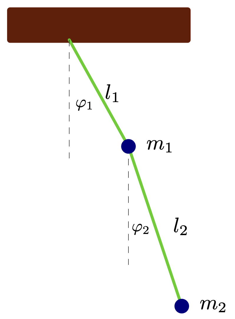
Thus, the stationary points of the double pendulum are given by:
%22%2F%3E%3Cuse%20xlink%3Ahref%3D%22%23b%22%20class%3D%22typst-text%22%20transform%3D%22matrix(1%200%200%20-1%2019.81%2019.87)%22%2F%3E%3Cuse%20xlink%3Ahref%3D%22%23c%22%20class%3D%22typst-text%22%20transform%3D%22matrix(1%200%200%20-1%2030.791%2016.165)%22%2F%3E%3Cuse%20xlink%3Ahref%3D%22%23d%22%20class%3D%22typst-text%22%20transform%3D%22matrix(1%200%200%20-1%2046.628%2016.165)%22%2F%3E%3C%2Fg%3E%3Cg%20class%3D%22typst-group%22%3E%3Cuse%20xlink%3Ahref%3D%22%23a%22%20class%3D%22typst-text%22%20transform%3D%22matrix(1%200%200%20-1%2010%2039.61)%22%2F%3E%3Cuse%20xlink%3Ahref%3D%22%23e%22%20class%3D%22typst-text%22%20transform%3D%22matrix(1%200%200%20-1%2019.81%2043.315)%22%2F%3E%3Cuse%20xlink%3Ahref%3D%22%23c%22%20class%3D%22typst-text%22%20transform%3D%22matrix(1%200%200%20-1%2030.791%2039.61)%22%2F%3E%3Cuse%20xlink%3Ahref%3D%22%23d%22%20class%3D%22typst-text%22%20transform%3D%22matrix(1%200%200%20-1%2046.628%2039.61)%22%2F%3E%3C%2Fg%3E%3C%2Fg%3E%3C%2Fg%3E%3C%2Fg%3E%3C%2Fg%3E%3Cdefs%3E%3Csymbol%20id%3D%22a%22%20overflow%3D%22visible%22%3E%3Cpath%20d%3D%22M7.545%206.63c-.255%200-.48-.045-.705-.12-.945-.315-1.605-1.245-1.98-2.1-.63-1.395-.81-1.965-1.275-3.54C2.04%201.185%201.26%201.89%201.26%203c0%201.005.705%202.46%201.2%203.03q.135.157.135.225c0%20.135-.075.21-.24.21q-.382%200-.99-1.305C.96%204.29.75%203.51.75%202.835c0-1.56%201.185-2.55%202.55-2.88l-.765-2.43a1.3%201.3%200%200%201-.09-.315c0-.315.165-.48.495-.48.285%200%20.48.15.6.435L4.05-.18c.165-.015.3-.015.435-.015%201.23%200%202.325.48%203.315%201.44q1.485%201.44%201.485%203.285c0%201.17-.615%202.1-1.74%202.1m1.2-2.43c0-.945-.45-1.77-1.365-2.475C6.525%201.095%205.61.78%204.62.78c-.09%200-.18%200-.255.015-.09%200-.135%200-.135-.015.225%201.185.36%201.89.42%202.1.345%201.185%201.365%202.775%202.745%202.775.84%200%201.35-.6%201.35-1.455%22%2F%3E%3C%2Fsymbol%3E%3Csymbol%20id%3D%22b%22%20overflow%3D%22visible%22%3E%3Cpath%20d%3D%22M3.182%206.972c-.452-.441-1.124-.662-2.037-.662v-.46c.619%200%201.112.094%201.49.272V.894c0-.137-.01-.221-.041-.263q-.08-.176-.945-.178h-.431V0l1.869.042L4.967%200v.452h-.431q-.864.002-.955.178c-.022.042-.032.126-.032.262v5.744c0%20.284-.042.336-.367.336%22%2F%3E%3C%2Fsymbol%3E%3Csymbol%20id%3D%22c%22%20overflow%3D%22visible%22%3E%3Cpath%20d%3D%22M10.47%205.505H1.2c-.24%200-.36-.12-.36-.345s.12-.345.36-.345h9.27c.24%200%20.36.12.36.345%200%20.18-.165.345-.36.345m0-2.82H1.2c-.24%200-.36-.12-.36-.345s.12-.345.36-.345h9.27c.24%200%20.36.12.36.345a.35.35%200%200%201-.36.345%22%2F%3E%3C%2Fsymbol%3E%3Csymbol%20id%3D%22d%22%20overflow%3D%22visible%22%3E%3Cpath%20d%3D%22M3.735-.33C5.85-.33%206.9%201.38%206.9%204.8c0%202.295-.48%203.825-1.425%204.575-.525.405-1.11.615-1.725.615C1.635%209.99.585%208.265.585%204.8c0-2.76.735-5.13%203.15-5.13m1.68%208.19c.105-.525.15-1.485.15-2.88%200-1.38-.06-2.4-.165-3.06Q5.107.12%203.735.12c-.345%200-.69.135-1.005.39-.405.345-.645%201.05-.75%202.13-.045.375-.06%201.155-.06%202.34%200%201.305.045%202.22.12%202.715.135.825.405%201.35.825%201.575.33.18.615.27.87.27.975%200%201.515-.795%201.68-1.68%22%2F%3E%3C%2Fsymbol%3E%3Csymbol%20id%3D%22e%22%20overflow%3D%22visible%22%3E%3Cpath%20d%3D%22M1.25%204.452c.335%200%20.587.252.587.588%200%20.378-.199.577-.587.588.23.494.756.892%201.438.892.924%200%201.533-.692%201.533-1.616%200-.505-.178-.988-.546-1.46a5%205%200%200%200-.41-.504L.777.473C.64.347.661.315.661%200h4.326l.326%201.974h-.441c-.074-.556-.157-.882-.252-.955-.053-.032-.378-.053-.997-.053H1.837c.704.62%201.355%201.176%201.974%201.67.473.367.809.692%201.019.976q.473.614.473%201.292c0%20.65-.252%201.165-.767%201.543-.451.346-1.018.525-1.69.525a2.36%202.36%200%200%201-1.502-.504c-.452-.367-.683-.83-.683-1.396%200-.357.263-.62.589-.62%22%2F%3E%3C%2Fsymbol%3E%3C%2Fdefs%3E%3C%2Fsvg%3E)
If we set the suspension point as the origin %22%2F%3E%3Cuse%20xlink%3Ahref%3D%22%23b%22%20class%3D%22typst-text%22%20transform%3D%22matrix(1%200%200%20-1%206.835%2012.22)%22%2F%3E%3Cuse%20xlink%3Ahref%3D%22%23c%22%20class%3D%22typst-text%22%20transform%3D%22matrix(1%200%200%20-1%2014.335%2012.22)%22%2F%3E%3Cuse%20xlink%3Ahref%3D%22%23b%22%20class%3D%22typst-text%22%20transform%3D%22matrix(1%200%200%20-1%2021.005%2012.22)%22%2F%3E%3Cuse%20xlink%3Ahref%3D%22%23d%22%20class%3D%22typst-text%22%20transform%3D%22matrix(1%200%200%20-1%2028.505%2012.22)%22%2F%3E%3C%2Fg%3E%3C%2Fg%3E%3Cdefs%3E%3Csymbol%20id%3D%22a%22%20overflow%3D%22visible%22%3E%3Cpath%20d%3D%22M4.77-3.72c.135%200%20.21.075.21.21%200%20.045-.03.105-.075.165-.78.6-1.41%201.59-1.875%202.955-.405%201.185-.615%202.355-.615%203.51v1.26c0%201.155.21%202.325.615%203.51.465%201.365%201.095%202.355%201.875%202.955a.24.24%200%200%201%20.075.165c0%20.135-.075.21-.21.21a.3.3%200%200%201-.105-.045c-.9-.69-1.65-1.71-2.265-3.075-.585-1.305-.885-2.535-.885-3.72V3.12c0-1.185.3-2.415.885-3.72.615-1.365%201.365-2.385%202.265-3.075a.3.3%200%200%201%20.105-.045%22%2F%3E%3C%2Fsymbol%3E%3Csymbol%20id%3D%22b%22%20overflow%3D%22visible%22%3E%3Cpath%20d%3D%22M3.735-.33C5.85-.33%206.9%201.38%206.9%204.8c0%202.295-.48%203.825-1.425%204.575-.525.405-1.11.615-1.725.615C1.635%209.99.585%208.265.585%204.8c0-2.76.735-5.13%203.15-5.13m1.68%208.19c.105-.525.15-1.485.15-2.88%200-1.38-.06-2.4-.165-3.06Q5.107.12%203.735.12c-.345%200-.69.135-1.005.39-.405.345-.645%201.05-.75%202.13-.045.375-.06%201.155-.06%202.34%200%201.305.045%202.22.12%202.715.135.825.405%201.35.825%201.575.33.18.615.27.87.27.975%200%201.515-.795%201.68-1.68%22%2F%3E%3C%2Fsymbol%3E%3Csymbol%20id%3D%22c%22%20overflow%3D%22visible%22%3E%3Cpath%20d%3D%22M2.085%201.59c-.48%200-.795-.36-.795-.84%200-.45.345-.825.795-.825.21%200%20.39.06.525.195L2.625%200c0-.945-.315-1.755-.945-2.4-.105-.12-.165-.21-.165-.27%200-.15.06-.225.195-.225s.315.18.57.525c.51.72.765%201.515.765%202.37%200%20.795-.27%201.59-.96%201.59%22%2F%3E%3C%2Fsymbol%3E%3Csymbol%20id%3D%22d%22%20overflow%3D%22visible%22%3E%3Cpath%20d%3D%22M1.17-3.675c.9.69%201.65%201.71%202.265%203.075.585%201.305.885%202.535.885%203.72v1.26c0%201.185-.3%202.415-.885%203.72-.615%201.365-1.365%202.385-2.265%203.075a.3.3%200%200%201-.105.045c-.135%200-.21-.075-.21-.21%200-.06.03-.12.075-.165.78-.6%201.41-1.59%201.875-2.955.405-1.185.615-2.355.615-3.51V3.12c0-1.155-.21-2.325-.615-3.51C2.34-1.755%201.71-2.745.93-3.345c-.045-.06-.075-.12-.075-.165%200-.135.075-.21.21-.21.015%200%20.06.015.105.045%22%2F%3E%3C%2Fsymbol%3E%3C%2Fdefs%3E%3C%2Fsvg%3E) ,
then the position of the first mass is given by:
,
then the position of the first mass is given by:

And the position of the second mass is given by:

Thus, if we set %22%2F%3E%3Cuse%20xlink%3Ahref%3D%22%23b%22%20class%3D%22typst-text%22%20transform%3D%22matrix(1%200%200%20-1%2010.81%2011.335)%22%2F%3E%3C%2Fg%3E%3C%2Fg%3E%3Cdefs%3E%3Csymbol%20id%3D%22a%22%20overflow%3D%22visible%22%3E%3Cpath%20d%3D%22M7.545%206.63c-.255%200-.48-.045-.705-.12-.945-.315-1.605-1.245-1.98-2.1-.63-1.395-.81-1.965-1.275-3.54C2.04%201.185%201.26%201.89%201.26%203c0%201.005.705%202.46%201.2%203.03q.135.157.135.225c0%20.135-.075.21-.24.21q-.382%200-.99-1.305C.96%204.29.75%203.51.75%202.835c0-1.56%201.185-2.55%202.55-2.88l-.765-2.43a1.3%201.3%200%200%201-.09-.315c0-.315.165-.48.495-.48.285%200%20.48.15.6.435L4.05-.18c.165-.015.3-.015.435-.015%201.23%200%202.325.48%203.315%201.44q1.485%201.44%201.485%203.285c0%201.17-.615%202.1-1.74%202.1m1.2-2.43c0-.945-.45-1.77-1.365-2.475C6.525%201.095%205.61.78%204.62.78c-.09%200-.18%200-.255.015-.09%200-.135%200-.135-.015.225%201.185.36%201.89.42%202.1.345%201.185%201.365%202.775%202.745%202.775.84%200%201.35-.6%201.35-1.455%22%2F%3E%3C%2Fsymbol%3E%3Csymbol%20id%3D%22b%22%20overflow%3D%22visible%22%3E%3Cpath%20d%3D%22M3.182%206.972c-.452-.441-1.124-.662-2.037-.662v-.46c.619%200%201.112.094%201.49.272V.894c0-.137-.01-.221-.041-.263q-.08-.176-.945-.178h-.431V0l1.869.042L4.967%200v.452h-.431q-.864.002-.955.178c-.022.042-.032.126-.032.262v5.744c0%20.284-.042.336-.367.336%22%2F%3E%3C%2Fsymbol%3E%3C%2Fdefs%3E%3C%2Fsvg%3E) and
and %22%2F%3E%3Cuse%20xlink%3Ahref%3D%22%23b%22%20class%3D%22typst-text%22%20transform%3D%22matrix(1%200%200%20-1%2010.81%2011.335)%22%2F%3E%3C%2Fg%3E%3C%2Fg%3E%3Cdefs%3E%3Csymbol%20id%3D%22a%22%20overflow%3D%22visible%22%3E%3Cpath%20d%3D%22M7.545%206.63c-.255%200-.48-.045-.705-.12-.945-.315-1.605-1.245-1.98-2.1-.63-1.395-.81-1.965-1.275-3.54C2.04%201.185%201.26%201.89%201.26%203c0%201.005.705%202.46%201.2%203.03q.135.157.135.225c0%20.135-.075.21-.24.21q-.382%200-.99-1.305C.96%204.29.75%203.51.75%202.835c0-1.56%201.185-2.55%202.55-2.88l-.765-2.43a1.3%201.3%200%200%201-.09-.315c0-.315.165-.48.495-.48.285%200%20.48.15.6.435L4.05-.18c.165-.015.3-.015.435-.015%201.23%200%202.325.48%203.315%201.44q1.485%201.44%201.485%203.285c0%201.17-.615%202.1-1.74%202.1m1.2-2.43c0-.945-.45-1.77-1.365-2.475C6.525%201.095%205.61.78%204.62.78c-.09%200-.18%200-.255.015-.09%200-.135%200-.135-.015.225%201.185.36%201.89.42%202.1.345%201.185%201.365%202.775%202.745%202.775.84%200%201.35-.6%201.35-1.455%22%2F%3E%3C%2Fsymbol%3E%3Csymbol%20id%3D%22b%22%20overflow%3D%22visible%22%3E%3Cpath%20d%3D%22M1.25%204.452c.335%200%20.587.252.587.588%200%20.378-.199.577-.587.588.23.494.756.892%201.438.892.924%200%201.533-.692%201.533-1.616%200-.505-.178-.988-.546-1.46a5%205%200%200%200-.41-.504L.777.473C.64.347.661.315.661%200h4.326l.326%201.974h-.441c-.074-.556-.157-.882-.252-.955-.053-.032-.378-.053-.997-.053H1.837c.704.62%201.355%201.176%201.974%201.67.473.367.809.692%201.019.976q.473.614.473%201.292c0%20.65-.252%201.165-.767%201.543-.451.346-1.018.525-1.69.525a2.36%202.36%200%200%201-1.502-.504c-.452-.367-.683-.83-.683-1.396%200-.357.263-.62.589-.62%22%2F%3E%3C%2Fsymbol%3E%3C%2Fdefs%3E%3C%2Fsvg%3E) close to the stationary point, the kinetic energy of the double pendulum is given by:
close to the stationary point, the kinetic energy of the double pendulum is given by:

The potential energy of the double pendulum is given by:

0.7 Normal Modes
As in Small Oscillations in General,
we can express the kinetic and potential energy of the system in terms of symmetric matrices and :

Thus, the general momentum of the system is given by:
%22%2F%3E%3Cuse%20xlink%3Ahref%3D%22%23b%22%20class%3D%22typst-text%22%20transform%3D%22matrix(1%200%200%20-1%2021.937%2030.895)%22%2F%3E%3Cg%20class%3D%22typst-group%22%3E%3Cuse%20xlink%3Ahref%3D%22%23c%22%20class%3D%22typst-text%22%20transform%3D%22matrix(1%200%200%20-1%2039.273%2020.74)%22%2F%3E%3Cuse%20xlink%3Ahref%3D%22%23d%22%20class%3D%22typst-text%22%20transform%3D%22matrix(1%200%200%20-1%2048.183%2020.74)%22%2F%3E%3Cuse%20xlink%3Ahref%3D%22%23c%22%20class%3D%22typst-text%22%20transform%3D%22matrix(1%200%200%20-1%2040.78%2041.185)%22%2F%3E%3Cuse%20xlink%3Ahref%3D%22%23e%22%20class%3D%22typst-text%22%20transform%3D%22matrix(1%200%200%20-1%2057.88%2041.305)%22%2F%3E%3Cuse%20xlink%3Ahref%3D%22%23f%22%20class%3D%22typst-text%22%20transform%3D%22matrix(1%200%200%20-1%2049.69%2041.185)%22%2F%3E%3Cpath%20fill%3D%22none%22%20stroke%3D%22%23000%22%20stroke-width%3D%22.72%22%20d%3D%22M39.273%2027.145h19.125%22%20class%3D%22typst-shape%22%2F%3E%3C%2Fg%3E%3Cuse%20xlink%3Ahref%3D%22%23b%22%20class%3D%22typst-text%22%20transform%3D%22matrix(1%200%200%20-1%2064.065%2030.895)%22%2F%3E%3Cuse%20xlink%3Ahref%3D%22%23g%22%20class%3D%22typst-text%22%20transform%3D%22matrix(1%200%200%20-1%2079.902%2030.895)%22%2F%3E%3Cuse%20xlink%3Ahref%3D%22%23e%22%20class%3D%22typst-text%22%20transform%3D%22matrix(1%200%200%20-1%20104.172%2031.015)%22%2F%3E%3Cuse%20xlink%3Ahref%3D%22%23f%22%20class%3D%22typst-text%22%20transform%3D%22matrix(1%200%200%20-1%2095.982%2030.895)%22%2F%3E%3C%2Fg%3E%3C%2Fg%3E%3Cdefs%3E%3Csymbol%20id%3D%22a%22%20overflow%3D%22visible%22%3E%3Cpath%20d%3D%22M5.325%206.63c-.66%200-1.29-.345-1.905-1.035-.165.69-.63%201.035-1.365%201.035-.615%200-1.065-.495-1.38-1.47-.15-.495-.225-.78-.225-.87%200-.135.075-.21.24-.21a.27.27%200%200%201%20.165.045c.075.135.12.24.135.345.27%201.14.615%201.71%201.02%201.71.27%200%20.405-.21.405-.615%200-.225-.03-.48-.105-.75L.66-1.77c-.135-.495-.15-.555-.735-.555-.27%200-.405-.12-.405-.345%200-.165.09-.24.255-.24.225%200%201.005.045%201.23.045.285%200%201.185-.045%201.47-.045.225%200%20.33.12.33.36%200%20.15-.135.225-.42.225-.27%200-.675-.015-.675.165%200%20.195.615%202.55.675%202.805.3-.555.75-.84%201.35-.84.975%200%201.83.495%202.58%201.5.69.915%201.035%201.89%201.035%202.895%200%201.305-.78%202.43-2.025%202.43m-.045-.45c.585%200%20.885-.45.885-1.335%200-.405-.09-.945-.255-1.62C5.565%201.92%205.13%201.065%204.605.63%204.29.375%204.005.24%203.72.24c-.435%200-.735.195-.9.6-.135.315-.21.54-.21.66l.765%203.135c.075.33.345.675.765%201.02s.795.525%201.14.525%22%2F%3E%3C%2Fsymbol%3E%3Csymbol%20id%3D%22b%22%20overflow%3D%22visible%22%3E%3Cpath%20d%3D%22M10.47%205.505H1.2c-.24%200-.36-.12-.36-.345s.12-.345.36-.345h9.27c.24%200%20.36.12.36.345%200%20.18-.165.345-.36.345m0-2.82H1.2c-.24%200-.36-.12-.36-.345s.12-.345.36-.345h9.27c.24%200%20.36.12.36.345a.35.35%200%200%201-.36.345%22%2F%3E%3C%2Fsymbol%3E%3Csymbol%20id%3D%22c%22%20overflow%3D%22visible%22%3E%3Cpath%20d%3D%22M3.84%208.61c0%20.345-.225.54-.66.57.465.705%201.14%201.065%202.025%201.065%201.38%200%202.055-1.155%202.055-2.625%200-.615-.12-1.365-.345-2.28-.255%201.035-.9%201.56-1.905%201.56-1.155%200-2.16-.48-3.06-1.41S.6%203.525.6%202.37c0-.555.195-1.125.585-1.695C1.65%200%202.37-.33%203.375-.33c1.35%200%202.475.63%203.36%201.905.84%201.23%201.755%203.36%201.755%205.265%200%201.065-.27%201.965-.81%202.685-.585.81-1.41%201.215-2.445%201.215-1.005%200-1.755-.345-2.265-1.05-.405-.555-.615-1.005-.615-1.35q0-.585.63-.585c.45%200%20.855.405.855.855m2.745-4.065c0-.945-.285-1.875-.87-2.79C5.07.72%204.305.21%203.42.21c-.99%200-1.56.645-1.56%201.605q0%20.63.315%201.755c.21.75.42%201.275.645%201.59.6.855%201.335%201.29%202.19%201.29%201.095%200%201.575-.81%201.575-1.905%22%2F%3E%3C%2Fsymbol%3E%3Csymbol%20id%3D%22d%22%20overflow%3D%22visible%22%3E%3Cpath%20d%3D%22M7.8%2010.005c0%20.165-.105.24-.3.24L5.31%2010.2l-1.965.045C3.12%2010.26%203%2010.14%203%209.885c0-.105.045-.18.135-.195.135-.015.255-.03.33-.03a6%206%200%200%200%20.795-.06c.075-.015.12-.06.12-.135%200-.03-.015-.12-.06-.27L2.34%201.23C2.25.9%202.1.705%201.875.63%201.785.6%201.515.585%201.05.585.735.585.585.465.585.225.585.075.735%200%201.05%200h6.855c.375%200%20.405%200%20.51.285l1.17%203.21c.045.105.06.18.06.225%200%20.15-.075.225-.24.225-.15%200-.225-.135-.3-.345-.285-.735-.555-1.29-.78-1.635-.555-.84-1.5-1.38-2.88-1.38H4.05c-.165%200-.27%200-.315.015-.105%200-.15.03-.15.075%200%20.03.03.135.075.33l1.995%208.01c.09.345.285.54.57.615.09.015.405.03.945.03.42%200%20.63%200%20.63.345%22%2F%3E%3C%2Fsymbol%3E%3Csymbol%20id%3D%22e%22%20overflow%3D%22visible%22%3E%3Cpath%20d%3D%22M-3.165%209.36a.8.8%200%200%201-.795.795.813.813%200%200%201-.81-.795.8.8%200%200%201%20.795-.795c.435%200%20.81.36.81.795%22%2F%3E%3C%2Fsymbol%3E%3Csymbol%20id%3D%22f%22%20overflow%3D%22visible%22%3E%3Cpath%20d%3D%22M5.58%205.655c-.3.645-.765.975-1.38.975-.975%200-1.83-.495-2.565-1.5C.945%204.2.6%203.24.6%202.235c0-1.305.75-2.43%201.995-2.43.54%200%201.08.255%201.635.765l-.615-2.46a.48.48%200%200%200-.39-.405%204%204%200%200%200-.615-.03c-.09-.015-.15-.015-.18-.015-.135-.015-.21-.135-.21-.345v-.06a.26.26%200%200%201%20.255-.165c.285%200%201.185.045%201.47.045s1.23-.045%201.515-.045q.315%200%20.315.36c0%20.15-.15.225-.435.225-.27%200-.645-.015-.645.165%200%20.06.015.165.06.315l2.025%208.25c0%20.135-.075.21-.21.21-.27%200-.84-.75-.99-.96m-.48-.06c.135-.315.21-.525.21-.66a2%202%200%200%200-.045-.24l-.36-1.455c-.285-1.08-.42-1.635-.435-1.665C4.185%201.05%203.36.24%202.64.24c-.585%200-.885.45-.885%201.335%200%20.69.465%202.37.675%202.925.285.705.945%201.68%201.77%201.68q.607%200%20.9-.585%22%2F%3E%3C%2Fsymbol%3E%3Csymbol%20id%3D%22g%22%20overflow%3D%22visible%22%3E%3Cpath%20d%3D%22M8.91.24C8.91.075%209%200%209.195%200l1.845.045C11.385.06%2012.6%200%2012.885%200c.225%200%20.345.12.345.36%200%20.15-.15.225-.465.225-.615%200-.915.06-.915.195%200%20.045.03.15.075.345l1.98%207.905c.075.315.225.51.42.585.09.03.36.045.795.045.375%200%20.54.015.54.36%200%20.15-.15.225-.465.225H13.23c-.435%200-.435-.03-.63-.315L7.26%201.62%206.12%209.855c-.06.375-.09.39-.525.39h-2.04c-.33%200-.495-.015-.495-.345%200-.165.165-.24.48-.24.3%200%20.915.045.915-.195%200-.03-.015-.12-.06-.27L2.505%201.65C2.37%201.08%202.025.735%201.5.63%201.125.585.63.645.63.24.63.075.72%200%20.9%200c.27%200%201.215.045%201.485.045C2.67.045%203.63%200%203.915%200c.225%200%20.33.12.33.36%200%20.135-.105.21-.33.225q-.945%200-.945.585c0%20.06.015.165.06.33l1.95%207.815L6.225.39C6.27.135%206.36%200%206.51%200c.12%200%20.24.105.375.3l5.835%209.105-2.04-8.175c-.09-.33-.24-.525-.465-.6-.09-.03-.375-.045-.84-.045-.315%200-.465-.03-.465-.345%22%2F%3E%3C%2Fsymbol%3E%3C%2Fdefs%3E%3C%2Fsvg%3E)
And the generalised force %22%2F%3E%3C%2Fg%3E%3C%2Fg%3E%3Cdefs%3E%3Csymbol%20id%3D%22a%22%20overflow%3D%22visible%22%3E%3Cpath%20d%3D%22M4.59-.36c.435%200%20.9.075%201.395.21-.045-.57-.06-.93-.06-1.065%200-1.125.435-1.695%201.29-1.695.915%200%201.62.735%201.965%201.41.375.78.57%201.29.57%201.53%200%20.135-.075.21-.225.21-.105%200-.18-.06-.225-.195-.225-.69-.84-1.395-1.68-1.395-.765%200-.87.615-.99%201.44%201.26.495%202.325%201.35%203.18%202.58s1.29%202.505%201.29%203.84c0%201.185-.345%202.145-1.05%202.91s-1.635%201.155-2.79%201.155c-.795%200-1.59-.195-2.385-.6-1.62-.795-2.805-2.055-3.57-3.75C.93%205.37.735%204.53.735%203.675.735%201.32%202.265-.36%204.59-.36m5.085%207.35c0-.915-.225-1.965-.675-3.18C8.475%202.415%207.665%201.38%206.54.72q-.09.495-.27.9-.293.675-1.08.675c-.825%200-1.575-.75-1.575-1.575%200-.135.015-.27.045-.375-1.005.465-1.5%201.41-1.5%202.85%200%20.63.12%201.395.375%202.295q.788%202.858%202.835%204.05.968.54%201.8.54c1.65%200%202.505-1.365%202.505-3.09M5.19%201.845c.555%200%20.84-.405.84-1.2%200-.135-.045-.21-.135-.24q-.63-.27-1.215-.27-.63%200-.63.585c0%20.57.57%201.125%201.14%201.125%22%2F%3E%3C%2Fsymbol%3E%3C%2Fdefs%3E%3C%2Fsvg%3E) of the system is given by:
of the system is given by:
%22%2F%3E%3Cuse%20xlink%3Ahref%3D%22%23b%22%20class%3D%22typst-text%22%20transform%3D%22matrix(1%200%200%20-1%2026.032%2030.895)%22%2F%3E%3Cuse%20xlink%3Ahref%3D%22%23c%22%20class%3D%22typst-text%22%20transform%3D%22matrix(1%200%200%20-1%2043.368%2020.74)%22%2F%3E%3Cuse%20xlink%3Ahref%3D%22%23d%22%20class%3D%22typst-text%22%20transform%3D%22matrix(1%200%200%20-1%2052.278%2020.74)%22%2F%3E%3Cuse%20xlink%3Ahref%3D%22%23c%22%20class%3D%22typst-text%22%20transform%3D%22matrix(1%200%200%20-1%2044.876%2041.185)%22%2F%3E%3Cuse%20xlink%3Ahref%3D%22%23e%22%20class%3D%22typst-text%22%20transform%3D%22matrix(1%200%200%20-1%2053.786%2041.185)%22%2F%3E%3Cpath%20fill%3D%22none%22%20stroke%3D%22%23000%22%20stroke-width%3D%22.72%22%20d%3D%22M43.368%2027.145h19.125%22%20class%3D%22typst-shape%22%2F%3E%3Cuse%20xlink%3Ahref%3D%22%23b%22%20class%3D%22typst-text%22%20transform%3D%22matrix(1%200%200%20-1%2068.16%2030.895)%22%2F%3E%3Cuse%20xlink%3Ahref%3D%22%23f%22%20class%3D%22typst-text%22%20transform%3D%22matrix(1%200%200%20-1%2083.997%2030.895)%22%2F%3E%3Cuse%20xlink%3Ahref%3D%22%23g%22%20class%3D%22typst-text%22%20transform%3D%22matrix(1%200%200%20-1%2097.752%2030.895)%22%2F%3E%3Cuse%20xlink%3Ahref%3D%22%23e%22%20class%3D%22typst-text%22%20transform%3D%22matrix(1%200%200%20-1%20103.587%2030.895)%22%2F%3E%3Cuse%20xlink%3Ahref%3D%22%23h%22%20class%3D%22typst-text%22%20transform%3D%22matrix(1%200%200%20-1%20114.12%2030.895)%22%2F%3E%3Cuse%20xlink%3Ahref%3D%22%23e%22%20class%3D%22typst-text%22%20transform%3D%22matrix(1%200%200%20-1%20129.123%2030.895)%22%2F%3E%3Cuse%20xlink%3Ahref%3D%22%23i%22%20class%3D%22typst-text%22%20transform%3D%22matrix(1%200%200%20-1%20135.813%2034.6)%22%2F%3E%3Cuse%20xlink%3Ahref%3D%22%23j%22%20class%3D%22typst-text%22%20transform%3D%22matrix(1%200%200%20-1%20142.628%2030.895)%22%2F%3E%3C%2Fg%3E%3C%2Fg%3E%3Cdefs%3E%3Csymbol%20id%3D%22a%22%20overflow%3D%22visible%22%3E%3Cpath%20d%3D%22M4.59-.36c.435%200%20.9.075%201.395.21-.045-.57-.06-.93-.06-1.065%200-1.125.435-1.695%201.29-1.695.915%200%201.62.735%201.965%201.41.375.78.57%201.29.57%201.53%200%20.135-.075.21-.225.21-.105%200-.18-.06-.225-.195-.225-.69-.84-1.395-1.68-1.395-.765%200-.87.615-.99%201.44%201.26.495%202.325%201.35%203.18%202.58s1.29%202.505%201.29%203.84c0%201.185-.345%202.145-1.05%202.91s-1.635%201.155-2.79%201.155c-.795%200-1.59-.195-2.385-.6-1.62-.795-2.805-2.055-3.57-3.75C.93%205.37.735%204.53.735%203.675.735%201.32%202.265-.36%204.59-.36m5.085%207.35c0-.915-.225-1.965-.675-3.18C8.475%202.415%207.665%201.38%206.54.72q-.09.495-.27.9-.293.675-1.08.675c-.825%200-1.575-.75-1.575-1.575%200-.135.015-.27.045-.375-1.005.465-1.5%201.41-1.5%202.85%200%20.63.12%201.395.375%202.295q.788%202.858%202.835%204.05.968.54%201.8.54c1.65%200%202.505-1.365%202.505-3.09M5.19%201.845c.555%200%20.84-.405.84-1.2%200-.135-.045-.21-.135-.24q-.63-.27-1.215-.27-.63%200-.63.585c0%20.57.57%201.125%201.14%201.125%22%2F%3E%3C%2Fsymbol%3E%3Csymbol%20id%3D%22b%22%20overflow%3D%22visible%22%3E%3Cpath%20d%3D%22M10.47%205.505H1.2c-.24%200-.36-.12-.36-.345s.12-.345.36-.345h9.27c.24%200%20.36.12.36.345%200%20.18-.165.345-.36.345m0-2.82H1.2c-.24%200-.36-.12-.36-.345s.12-.345.36-.345h9.27c.24%200%20.36.12.36.345a.35.35%200%200%201-.36.345%22%2F%3E%3C%2Fsymbol%3E%3Csymbol%20id%3D%22c%22%20overflow%3D%22visible%22%3E%3Cpath%20d%3D%22M3.84%208.61c0%20.345-.225.54-.66.57.465.705%201.14%201.065%202.025%201.065%201.38%200%202.055-1.155%202.055-2.625%200-.615-.12-1.365-.345-2.28-.255%201.035-.9%201.56-1.905%201.56-1.155%200-2.16-.48-3.06-1.41S.6%203.525.6%202.37c0-.555.195-1.125.585-1.695C1.65%200%202.37-.33%203.375-.33c1.35%200%202.475.63%203.36%201.905.84%201.23%201.755%203.36%201.755%205.265%200%201.065-.27%201.965-.81%202.685-.585.81-1.41%201.215-2.445%201.215-1.005%200-1.755-.345-2.265-1.05-.405-.555-.615-1.005-.615-1.35q0-.585.63-.585c.45%200%20.855.405.855.855m2.745-4.065c0-.945-.285-1.875-.87-2.79C5.07.72%204.305.21%203.42.21c-.99%200-1.56.645-1.56%201.605q0%20.63.315%201.755c.21.75.42%201.275.645%201.59.6.855%201.335%201.29%202.19%201.29%201.095%200%201.575-.81%201.575-1.905%22%2F%3E%3C%2Fsymbol%3E%3Csymbol%20id%3D%22d%22%20overflow%3D%22visible%22%3E%3Cpath%20d%3D%22M7.8%2010.005c0%20.165-.105.24-.3.24L5.31%2010.2l-1.965.045C3.12%2010.26%203%2010.14%203%209.885c0-.105.045-.18.135-.195.135-.015.255-.03.33-.03a6%206%200%200%200%20.795-.06c.075-.015.12-.06.12-.135%200-.03-.015-.12-.06-.27L2.34%201.23C2.25.9%202.1.705%201.875.63%201.785.6%201.515.585%201.05.585.735.585.585.465.585.225.585.075.735%200%201.05%200h6.855c.375%200%20.405%200%20.51.285l1.17%203.21c.045.105.06.18.06.225%200%20.15-.075.225-.24.225-.15%200-.225-.135-.3-.345-.285-.735-.555-1.29-.78-1.635-.555-.84-1.5-1.38-2.88-1.38H4.05c-.165%200-.27%200-.315.015-.105%200-.15.03-.15.075%200%20.03.03.135.075.33l1.995%208.01c.09.345.285.54.57.615.09.015.405.03.945.03.42%200%20.63%200%20.63.345%22%2F%3E%3C%2Fsymbol%3E%3Csymbol%20id%3D%22e%22%20overflow%3D%22visible%22%3E%3Cpath%20d%3D%22M5.58%205.655c-.3.645-.765.975-1.38.975-.975%200-1.83-.495-2.565-1.5C.945%204.2.6%203.24.6%202.235c0-1.305.75-2.43%201.995-2.43.54%200%201.08.255%201.635.765l-.615-2.46a.48.48%200%200%200-.39-.405%204%204%200%200%200-.615-.03c-.09-.015-.15-.015-.18-.015-.135-.015-.21-.135-.21-.345v-.06a.26.26%200%200%201%20.255-.165c.285%200%201.185.045%201.47.045s1.23-.045%201.515-.045q.315%200%20.315.36c0%20.15-.15.225-.435.225-.27%200-.645-.015-.645.165%200%20.06.015.165.06.315l2.025%208.25c0%20.135-.075.21-.21.21-.27%200-.84-.75-.99-.96m-.48-.06c.135-.315.21-.525.21-.66a2%202%200%200%200-.045-.24l-.36-1.455c-.285-1.08-.42-1.635-.435-1.665C4.185%201.05%203.36.24%202.64.24c-.585%200-.885.45-.885%201.335%200%20.69.465%202.37.675%202.925.285.705.945%201.68%201.77%201.68q.607%200%20.9-.585%22%2F%3E%3C%2Fsymbol%3E%3Csymbol%20id%3D%22f%22%20overflow%3D%22visible%22%3E%3Cpath%20d%3D%22M12.06%2010.2c-.315%200-1.335.045-1.65.045-.225%200-.345-.12-.345-.36%200-.12.105-.195.315-.24s.33-.12.33-.225c0-.165-.165-.39-.51-.645L4.53%204.44l1.155%204.59q.113.472.405.585c.09.03.345.045.78.045.39%200%20.57%200%20.57.36q0%20.225-.27.225L5.265%2010.2l-1.92.045c-.24.015-.36-.105-.36-.345%200-.165.165-.24.495-.24.3%200%20.915.045.915-.195%200-.03-.015-.12-.06-.27L2.34%201.23C2.265.9%202.115.705%201.89.63%201.785.6%201.515.585%201.05.585.72.585.57.555.57.24.57.075.66%200%20.855%200l1.89.045L3.69.03c.165%200%20.795-.03.96-.03q.36%200%20.36.36c0%20.15-.15.225-.465.225-.615%200-.915.06-.915.195%200%20.075.045.3.135.645l.585%202.31%202.145%201.65L8.19%201.47c.105-.255.165-.42.165-.495%200-.255-.24-.39-.705-.39-.27%200-.39-.06-.39-.36Q7.26%200%207.53%200c.33%200%201.47.045%201.8.045C9.615.045%2010.515%200%2010.8%200q.315%200%20.315.36c0%20.135-.12.21-.345.225-.615%200-.765.165-.975.63L7.68%206.06c-.015.075-.045.135-.06.18l3%202.31c.735.57%201.365.915%201.875%201.035.36.06.84.045.84.435q0%20.225-.225.225c-.21%200-.84-.045-1.05-.045%22%2F%3E%3C%2Fsymbol%3E%3Csymbol%20id%3D%22g%22%20overflow%3D%22visible%22%3E%3Cpath%20d%3D%22M4.77-3.72c.135%200%20.21.075.21.21%200%20.045-.03.105-.075.165-.78.6-1.41%201.59-1.875%202.955-.405%201.185-.615%202.355-.615%203.51v1.26c0%201.155.21%202.325.615%203.51.465%201.365%201.095%202.355%201.875%202.955a.24.24%200%200%201%20.075.165c0%20.135-.075.21-.21.21a.3.3%200%200%201-.105-.045c-.9-.69-1.65-1.71-2.265-3.075-.585-1.305-.885-2.535-.885-3.72V3.12c0-1.185.3-2.415.885-3.72.615-1.365%201.365-2.385%202.265-3.075a.3.3%200%200%201%20.105-.045%22%2F%3E%3C%2Fsymbol%3E%3Csymbol%20id%3D%22h%22%20overflow%3D%22visible%22%3E%3Cpath%20d%3D%22M10.47%204.05H1.2c-.24%200-.36-.105-.36-.3s.12-.3.36-.3h9.27c.24%200%20.36.105.36.3%200%20.18-.18.3-.36.3%22%2F%3E%3C%2Fsymbol%3E%3Csymbol%20id%3D%22i%22%20overflow%3D%22visible%22%3E%3Cpath%20d%3D%22M5.418%203.35c0%201.186-.21%202.089-.62%202.709-.335.524-1.007.913-1.816.913-.336%200-.64-.053-.903-.168C.924%206.321.546%204.977.546%203.349c0-.357.021-.693.052-1.018C.778.956%201.418-.21%202.983-.21c.336%200%20.64.052.903.168C5.04.431%205.418%201.743%205.418%203.349M4.221%205.68c.115-.388.178-1.112.178-2.194%200-1.029-.042-1.754-.136-2.184C4.137.682%203.696.168%202.982.168c-.263%200-.525.084-.767.262-.325.242-.524.715-.608%201.439-.032.241-.042.777-.042%201.617%200%201.019.052%201.722.157%202.1q.268%201.008%201.26%201.008c.63%200%201.092-.41%201.239-.913%22%2F%3E%3C%2Fsymbol%3E%3Csymbol%20id%3D%22j%22%20overflow%3D%22visible%22%3E%3Cpath%20d%3D%22M1.17-3.675c.9.69%201.65%201.71%202.265%203.075.585%201.305.885%202.535.885%203.72v1.26c0%201.185-.3%202.415-.885%203.72-.615%201.365-1.365%202.385-2.265%203.075a.3.3%200%200%201-.105.045c-.135%200-.21-.075-.21-.21%200-.06.03-.12.075-.165.78-.6%201.41-1.59%201.875-2.955.405-1.185.615-2.355.615-3.51V3.12c0-1.155-.21-2.325-.615-3.51C2.34-1.755%201.71-2.745.93-3.345c-.045-.06-.075-.12-.075-.165%200-.135.075-.21.21-.21.015%200%20.06.015.105.045%22%2F%3E%3C%2Fsymbol%3E%3C%2Fdefs%3E%3C%2Fsvg%3E)
And the Euler-Lagrange equation is given by:

As, is a positive definite symmetric matrix,
the inverse of exists.
Thus, the equation of motion of the system can be expressed as:
%22%2F%3E%3Cuse%20xlink%3Ahref%3D%22%23b%22%20class%3D%22typst-text%22%20transform%3D%22matrix(1%200%200%20-1%2010%2022.417)%22%2F%3E%3Cuse%20xlink%3Ahref%3D%22%23c%22%20class%3D%22typst-text%22%20transform%3D%22matrix(1%200%200%20-1%2020.533%2022.417)%22%2F%3E%3Cuse%20xlink%3Ahref%3D%22%23d%22%20class%3D%22typst-text%22%20transform%3D%22matrix(1%200%200%20-1%2035.537%2022.417)%22%2F%3E%3Cuse%20xlink%3Ahref%3D%22%23e%22%20class%3D%22typst-text%22%20transform%3D%22matrix(1%200%200%20-1%2051.617%2016.972)%22%2F%3E%3Cuse%20xlink%3Ahref%3D%22%23f%22%20class%3D%22typst-text%22%20transform%3D%22matrix(1%200%200%20-1%2059.786%2016.972)%22%2F%3E%3Cuse%20xlink%3Ahref%3D%22%23g%22%20class%3D%22typst-text%22%20transform%3D%22matrix(1%200%200%20-1%2066.6%2022.417)%22%2F%3E%3Cuse%20xlink%3Ahref%3D%22%23h%22%20class%3D%22typst-text%22%20transform%3D%22matrix(1%200%200%20-1%2080.355%2022.417)%22%2F%3E%3Cuse%20xlink%3Ahref%3D%22%23b%22%20class%3D%22typst-text%22%20transform%3D%22matrix(1%200%200%20-1%2086.19%2022.417)%22%2F%3E%3Cuse%20xlink%3Ahref%3D%22%23i%22%20class%3D%22typst-text%22%20transform%3D%22matrix(1%200%200%20-1%2096.724%2022.417)%22%2F%3E%3Cuse%20xlink%3Ahref%3D%22%23b%22%20class%3D%22typst-text%22%20transform%3D%22matrix(1%200%200%20-1%20111.727%2022.417)%22%2F%3E%3Cuse%20xlink%3Ahref%3D%22%23j%22%20class%3D%22typst-text%22%20transform%3D%22matrix(1%200%200%20-1%20118.417%2026.122)%22%2F%3E%3Cuse%20xlink%3Ahref%3D%22%23k%22%20class%3D%22typst-text%22%20transform%3D%22matrix(1%200%200%20-1%20125.231%2022.417)%22%2F%3E%3Cuse%20xlink%3Ahref%3D%22%23l%22%20class%3D%22typst-text%22%20transform%3D%22matrix(1%200%200%20-1%20135.233%2022.417)%22%2F%3E%3Cuse%20xlink%3Ahref%3D%22%23m%22%20class%3D%22typst-text%22%20transform%3D%22matrix(1%200%200%20-1%20151.07%2022.417)%22%2F%3E%3C%2Fg%3E%3C%2Fg%3E%3Cdefs%3E%3Csymbol%20id%3D%22a%22%20overflow%3D%22visible%22%3E%3Cpath%20d%3D%22M-1.89%209.375c0%20.39-.375.705-.765.705s-.765-.315-.765-.705.36-.72.75-.72c.435%200%20.78.3.78.72m-2.595%200c0%20.39-.36.705-.75.705-.405%200-.78-.3-.78-.705s.36-.72.765-.72c.42%200%20.765.3.765.72%22%2F%3E%3C%2Fsymbol%3E%3Csymbol%20id%3D%22b%22%20overflow%3D%22visible%22%3E%3Cpath%20d%3D%22M5.58%205.655c-.3.645-.765.975-1.38.975-.975%200-1.83-.495-2.565-1.5C.945%204.2.6%203.24.6%202.235c0-1.305.75-2.43%201.995-2.43.54%200%201.08.255%201.635.765l-.615-2.46a.48.48%200%200%200-.39-.405%204%204%200%200%200-.615-.03c-.09-.015-.15-.015-.18-.015-.135-.015-.21-.135-.21-.345v-.06a.26.26%200%200%201%20.255-.165c.285%200%201.185.045%201.47.045s1.23-.045%201.515-.045q.315%200%20.315.36c0%20.15-.15.225-.435.225-.27%200-.645-.015-.645.165%200%20.06.015.165.06.315l2.025%208.25c0%20.135-.075.21-.21.21-.27%200-.84-.75-.99-.96m-.48-.06c.135-.315.21-.525.21-.66a2%202%200%200%200-.045-.24l-.36-1.455c-.285-1.08-.42-1.635-.435-1.665C4.185%201.05%203.36.24%202.64.24c-.585%200-.885.45-.885%201.335%200%20.69.465%202.37.675%202.925.285.705.945%201.68%201.77%201.68q.607%200%20.9-.585%22%2F%3E%3C%2Fsymbol%3E%3Csymbol%20id%3D%22c%22%20overflow%3D%22visible%22%3E%3Cpath%20d%3D%22M10.47%204.11H6.195v4.275q0%20.36-.36.36t-.36-.36V4.11H1.2q-.36%200-.36-.36t.36-.36h4.275V-.885q0-.36.36-.36t.36.36V3.39h4.275q.36%200%20.36.36c0%20.195-.165.36-.36.36%22%2F%3E%3C%2Fsymbol%3E%3Csymbol%20id%3D%22d%22%20overflow%3D%22visible%22%3E%3Cpath%20d%3D%22M8.91.24C8.91.075%209%200%209.195%200l1.845.045C11.385.06%2012.6%200%2012.885%200c.225%200%20.345.12.345.36%200%20.15-.15.225-.465.225-.615%200-.915.06-.915.195%200%20.045.03.15.075.345l1.98%207.905c.075.315.225.51.42.585.09.03.36.045.795.045.375%200%20.54.015.54.36%200%20.15-.15.225-.465.225H13.23c-.435%200-.435-.03-.63-.315L7.26%201.62%206.12%209.855c-.06.375-.09.39-.525.39h-2.04c-.33%200-.495-.015-.495-.345%200-.165.165-.24.48-.24.3%200%20.915.045.915-.195%200-.03-.015-.12-.06-.27L2.505%201.65C2.37%201.08%202.025.735%201.5.63%201.125.585.63.645.63.24.63.075.72%200%20.9%200c.27%200%201.215.045%201.485.045C2.67.045%203.63%200%203.915%200c.225%200%20.33.12.33.36%200%20.135-.105.21-.33.225q-.945%200-.945.585c0%20.06.015.165.06.33l1.95%207.815L6.225.39C6.27.135%206.36%200%206.51%200c.12%200%20.24.105.375.3l5.835%209.105-2.04-8.175c-.09-.33-.24-.525-.465-.6-.09-.03-.375-.045-.84-.045-.315%200-.465-.03-.465-.345%22%2F%3E%3C%2Fsymbol%3E%3Csymbol%20id%3D%22e%22%20overflow%3D%22visible%22%3E%3Cpath%20d%3D%22M7.308%202.867H.861c-.21%200-.273-.106-.273-.242%200-.137.063-.242.273-.242h6.447c.21%200%20.273.105.273.242%200%20.126-.063.241-.273.241%22%2F%3E%3C%2Fsymbol%3E%3Csymbol%20id%3D%22f%22%20overflow%3D%22visible%22%3E%3Cpath%20d%3D%22M3.182%206.972c-.452-.441-1.124-.662-2.037-.662v-.46c.619%200%201.112.094%201.49.272V.894c0-.137-.01-.221-.041-.263q-.08-.176-.945-.178h-.431V0l1.869.042L4.967%200v.452h-.431q-.864.002-.955.178c-.022.042-.032.126-.032.262v5.744c0%20.284-.042.336-.367.336%22%2F%3E%3C%2Fsymbol%3E%3Csymbol%20id%3D%22g%22%20overflow%3D%22visible%22%3E%3Cpath%20d%3D%22M12.06%2010.2c-.315%200-1.335.045-1.65.045-.225%200-.345-.12-.345-.36%200-.12.105-.195.315-.24s.33-.12.33-.225c0-.165-.165-.39-.51-.645L4.53%204.44l1.155%204.59q.113.472.405.585c.09.03.345.045.78.045.39%200%20.57%200%20.57.36q0%20.225-.27.225L5.265%2010.2l-1.92.045c-.24.015-.36-.105-.36-.345%200-.165.165-.24.495-.24.3%200%20.915.045.915-.195%200-.03-.015-.12-.06-.27L2.34%201.23C2.265.9%202.115.705%201.89.63%201.785.6%201.515.585%201.05.585.72.585.57.555.57.24.57.075.66%200%20.855%200l1.89.045L3.69.03c.165%200%20.795-.03.96-.03q.36%200%20.36.36c0%20.15-.15.225-.465.225-.615%200-.915.06-.915.195%200%20.075.045.3.135.645l.585%202.31%202.145%201.65L8.19%201.47c.105-.255.165-.42.165-.495%200-.255-.24-.39-.705-.39-.27%200-.39-.06-.39-.36Q7.26%200%207.53%200c.33%200%201.47.045%201.8.045C9.615.045%2010.515%200%2010.8%200q.315%200%20.315.36c0%20.135-.12.21-.345.225-.615%200-.765.165-.975.63L7.68%206.06c-.015.075-.045.135-.06.18l3%202.31c.735.57%201.365.915%201.875%201.035.36.06.84.045.84.435q0%20.225-.225.225c-.21%200-.84-.045-1.05-.045%22%2F%3E%3C%2Fsymbol%3E%3Csymbol%20id%3D%22h%22%20overflow%3D%22visible%22%3E%3Cpath%20d%3D%22M4.77-3.72c.135%200%20.21.075.21.21%200%20.045-.03.105-.075.165-.78.6-1.41%201.59-1.875%202.955-.405%201.185-.615%202.355-.615%203.51v1.26c0%201.155.21%202.325.615%203.51.465%201.365%201.095%202.355%201.875%202.955a.24.24%200%200%201%20.075.165c0%20.135-.075.21-.21.21a.3.3%200%200%201-.105-.045c-.9-.69-1.65-1.71-2.265-3.075-.585-1.305-.885-2.535-.885-3.72V3.12c0-1.185.3-2.415.885-3.72.615-1.365%201.365-2.385%202.265-3.075a.3.3%200%200%201%20.105-.045%22%2F%3E%3C%2Fsymbol%3E%3Csymbol%20id%3D%22i%22%20overflow%3D%22visible%22%3E%3Cpath%20d%3D%22M10.47%204.05H1.2c-.24%200-.36-.105-.36-.3s.12-.3.36-.3h9.27c.24%200%20.36.105.36.3%200%20.18-.18.3-.36.3%22%2F%3E%3C%2Fsymbol%3E%3Csymbol%20id%3D%22j%22%20overflow%3D%22visible%22%3E%3Cpath%20d%3D%22M5.418%203.35c0%201.186-.21%202.089-.62%202.709-.335.524-1.007.913-1.816.913-.336%200-.64-.053-.903-.168C.924%206.321.546%204.977.546%203.349c0-.357.021-.693.052-1.018C.778.956%201.418-.21%202.983-.21c.336%200%20.64.052.903.168C5.04.431%205.418%201.743%205.418%203.349M4.221%205.68c.115-.388.178-1.112.178-2.194%200-1.029-.042-1.754-.136-2.184C4.137.682%203.696.168%202.982.168c-.263%200-.525.084-.767.262-.325.242-.524.715-.608%201.439-.032.241-.042.777-.042%201.617%200%201.019.052%201.722.157%202.1q.268%201.008%201.26%201.008c.63%200%201.092-.41%201.239-.913%22%2F%3E%3C%2Fsymbol%3E%3Csymbol%20id%3D%22k%22%20overflow%3D%22visible%22%3E%3Cpath%20d%3D%22M1.17-3.675c.9.69%201.65%201.71%202.265%203.075.585%201.305.885%202.535.885%203.72v1.26c0%201.185-.3%202.415-.885%203.72-.615%201.365-1.365%202.385-2.265%203.075a.3.3%200%200%201-.105.045c-.135%200-.21-.075-.21-.21%200-.06.03-.12.075-.165.78-.6%201.41-1.59%201.875-2.955.405-1.185.615-2.355.615-3.51V3.12c0-1.155-.21-2.325-.615-3.51C2.34-1.755%201.71-2.745.93-3.345c-.045-.06-.075-.12-.075-.165%200-.135.075-.21.21-.21.015%200%20.06.015.105.045%22%2F%3E%3C%2Fsymbol%3E%3Csymbol%20id%3D%22l%22%20overflow%3D%22visible%22%3E%3Cpath%20d%3D%22M10.47%205.505H1.2c-.24%200-.36-.12-.36-.345s.12-.345.36-.345h9.27c.24%200%20.36.12.36.345%200%20.18-.165.345-.36.345m0-2.82H1.2c-.24%200-.36-.12-.36-.345s.12-.345.36-.345h9.27c.24%200%20.36.12.36.345a.35.35%200%200%201-.36.345%22%2F%3E%3C%2Fsymbol%3E%3Csymbol%20id%3D%22m%22%20overflow%3D%22visible%22%3E%3Cpath%20d%3D%22M3.735-.33C5.85-.33%206.9%201.38%206.9%204.8c0%202.295-.48%203.825-1.425%204.575-.525.405-1.11.615-1.725.615C1.635%209.99.585%208.265.585%204.8c0-2.76.735-5.13%203.15-5.13m1.68%208.19c.105-.525.15-1.485.15-2.88%200-1.38-.06-2.4-.165-3.06Q5.107.12%203.735.12c-.345%200-.69.135-1.005.39-.405.345-.645%201.05-.75%202.13-.045.375-.06%201.155-.06%202.34%200%201.305.045%202.22.12%202.715.135.825.405%201.35.825%201.575.33.18.615.27.87.27.975%200%201.515-.795%201.68-1.68%22%2F%3E%3C%2Fsymbol%3E%3C%2Fdefs%3E%3C%2Fsvg%3E)
A normal mode of the system is a solution of the above equation of the form:
%22%2F%3E%3Cuse%20xlink%3Ahref%3D%22%23b%22%20class%3D%22typst-text%22%20transform%3D%22matrix(1%200%200%20-1%2017.2%2021.22)%22%2F%3E%3Cuse%20xlink%3Ahref%3D%22%23c%22%20class%3D%22typst-text%22%20transform%3D%22matrix(1%200%200%20-1%2023.035%2021.22)%22%2F%3E%3Cuse%20xlink%3Ahref%3D%22%23d%22%20class%3D%22typst-text%22%20transform%3D%22matrix(1%200%200%20-1%2028.45%2021.22)%22%2F%3E%3Cuse%20xlink%3Ahref%3D%22%23e%22%20class%3D%22typst-text%22%20transform%3D%22matrix(1%200%200%20-1%2038.452%2021.22)%22%2F%3E%3Cuse%20xlink%3Ahref%3D%22%23a%22%20class%3D%22typst-text%22%20transform%3D%22matrix(1%200%200%20-1%2054.288%2021.22)%22%2F%3E%3Cuse%20xlink%3Ahref%3D%22%23f%22%20class%3D%22typst-text%22%20transform%3D%22matrix(1%200%200%20-1%2060.978%2024.925)%22%2F%3E%3Cuse%20xlink%3Ahref%3D%22%23g%22%20class%3D%22typst-text%22%20transform%3D%22matrix(1%200%200%20-1%2071.126%2021.22)%22%2F%3E%3Cuse%20xlink%3Ahref%3D%22%23h%22%20class%3D%22typst-text%22%20transform%3D%22matrix(1%200%200%20-1%2086.13%2021.22)%22%2F%3E%3Cuse%20xlink%3Ahref%3D%22%23b%22%20class%3D%22typst-text%22%20transform%3D%22matrix(1%200%200%20-1%2093%2021.22)%22%2F%3E%3Cuse%20xlink%3Ahref%3D%22%23c%22%20class%3D%22typst-text%22%20transform%3D%22matrix(1%200%200%20-1%2098.835%2021.22)%22%2F%3E%3Cuse%20xlink%3Ahref%3D%22%23d%22%20class%3D%22typst-text%22%20transform%3D%22matrix(1%200%200%20-1%20104.25%2021.22)%22%2F%3E%3Cuse%20xlink%3Ahref%3D%22%23i%22%20class%3D%22typst-text%22%20transform%3D%22matrix(1%200%200%20-1%20110.085%2021.22)%22%2F%3E%3C%2Fg%3E%3C%2Fg%3E%3Cdefs%3E%3Csymbol%20id%3D%22a%22%20overflow%3D%22visible%22%3E%3Cpath%20d%3D%22M5.58%205.655c-.3.645-.765.975-1.38.975-.975%200-1.83-.495-2.565-1.5C.945%204.2.6%203.24.6%202.235c0-1.305.75-2.43%201.995-2.43.54%200%201.08.255%201.635.765l-.615-2.46a.48.48%200%200%200-.39-.405%204%204%200%200%200-.615-.03c-.09-.015-.15-.015-.18-.015-.135-.015-.21-.135-.21-.345v-.06a.26.26%200%200%201%20.255-.165c.285%200%201.185.045%201.47.045s1.23-.045%201.515-.045q.315%200%20.315.36c0%20.15-.15.225-.435.225-.27%200-.645-.015-.645.165%200%20.06.015.165.06.315l2.025%208.25c0%20.135-.075.21-.21.21-.27%200-.84-.75-.99-.96m-.48-.06c.135-.315.21-.525.21-.66a2%202%200%200%200-.045-.24l-.36-1.455c-.285-1.08-.42-1.635-.435-1.665C4.185%201.05%203.36.24%202.64.24c-.585%200-.885.45-.885%201.335%200%20.69.465%202.37.675%202.925.285.705.945%201.68%201.77%201.68q.607%200%20.9-.585%22%2F%3E%3C%2Fsymbol%3E%3Csymbol%20id%3D%22b%22%20overflow%3D%22visible%22%3E%3Cpath%20d%3D%22M4.77-3.72c.135%200%20.21.075.21.21%200%20.045-.03.105-.075.165-.78.6-1.41%201.59-1.875%202.955-.405%201.185-.615%202.355-.615%203.51v1.26c0%201.155.21%202.325.615%203.51.465%201.365%201.095%202.355%201.875%202.955a.24.24%200%200%201%20.075.165c0%20.135-.075.21-.21.21a.3.3%200%200%201-.105-.045c-.9-.69-1.65-1.71-2.265-3.075-.585-1.305-.885-2.535-.885-3.72V3.12c0-1.185.3-2.415.885-3.72.615-1.365%201.365-2.385%202.265-3.075a.3.3%200%200%201%20.105-.045%22%2F%3E%3C%2Fsymbol%3E%3Csymbol%20id%3D%22c%22%20overflow%3D%22visible%22%3E%3Cpath%20d%3D%22M4.95%206.285c0%20.135-.15.21-.465.21H3.27q.585%202.34.585%202.43c0%20.315-.165.465-.48.465-.345%200-.555-.195-.645-.585l-.555-2.31H.84c-.33%200-.495-.015-.495-.33%200-.165.15-.24.465-.24h1.215C1.29%203%20.93%201.455.93%201.26c0-.84.57-1.425%201.41-1.425.57%200%201.065.255%201.5.78.36.435.615.855.78%201.26.06.165.09.255.09.3%200%20.135-.075.21-.225.21-.12%200-.21-.075-.27-.24C3.705.9%203.09.285%202.355.285c-.255%200-.39.21-.39.615%200%20.225.03.465.09.705l1.065%204.32h1.335c.39%200%20.495.03.495.36%22%2F%3E%3C%2Fsymbol%3E%3Csymbol%20id%3D%22d%22%20overflow%3D%22visible%22%3E%3Cpath%20d%3D%22M1.17-3.675c.9.69%201.65%201.71%202.265%203.075.585%201.305.885%202.535.885%203.72v1.26c0%201.185-.3%202.415-.885%203.72-.615%201.365-1.365%202.385-2.265%203.075a.3.3%200%200%201-.105.045c-.135%200-.21-.075-.21-.21%200-.06.03-.12.075-.165.78-.6%201.41-1.59%201.875-2.955.405-1.185.615-2.355.615-3.51V3.12c0-1.155-.21-2.325-.615-3.51C2.34-1.755%201.71-2.745.93-3.345c-.045-.06-.075-.12-.075-.165%200-.135.075-.21.21-.21.015%200%20.06.015.105.045%22%2F%3E%3C%2Fsymbol%3E%3Csymbol%20id%3D%22e%22%20overflow%3D%22visible%22%3E%3Cpath%20d%3D%22M10.47%205.505H1.2c-.24%200-.36-.12-.36-.345s.12-.345.36-.345h9.27c.24%200%20.36.12.36.345%200%20.18-.165.345-.36.345m0-2.82H1.2c-.24%200-.36-.12-.36-.345s.12-.345.36-.345h9.27c.24%200%20.36.12.36.345a.35.35%200%200%201-.36.345%22%2F%3E%3C%2Fsymbol%3E%3Csymbol%20id%3D%22f%22%20overflow%3D%22visible%22%3E%3Cpath%20d%3D%22M5.418%203.35c0%201.186-.21%202.089-.62%202.709-.335.524-1.007.913-1.816.913-.336%200-.64-.053-.903-.168C.924%206.321.546%204.977.546%203.349c0-.357.021-.693.052-1.018C.778.956%201.418-.21%202.983-.21c.336%200%20.64.052.903.168C5.04.431%205.418%201.743%205.418%203.349M4.221%205.68c.115-.388.178-1.112.178-2.194%200-1.029-.042-1.754-.136-2.184C4.137.682%203.696.168%202.982.168c-.263%200-.525.084-.767.262-.325.242-.524.715-.608%201.439-.032.241-.042.777-.042%201.617%200%201.019.052%201.722.157%202.1q.268%201.008%201.26%201.008c.63%200%201.092-.41%201.239-.913%22%2F%3E%3C%2Fsymbol%3E%3Csymbol%20id%3D%22g%22%20overflow%3D%22visible%22%3E%3Cpath%20d%3D%22M10.47%204.11H6.195v4.275q0%20.36-.36.36t-.36-.36V4.11H1.2q-.36%200-.36-.36t.36-.36h4.275V-.885q0-.36.36-.36t.36.36V3.39h4.275q.36%200%20.36.36c0%20.195-.165.36-.36.36%22%2F%3E%3C%2Fsymbol%3E%3Csymbol%20id%3D%22h%22%20overflow%3D%22visible%22%3E%3Cpath%20d%3D%22M4.92%204.875c0-.375.195-.57.6-.57.54%200%20.885.465.885%201.005%200%20.84-.885%201.32-1.785%201.32-1.035%200-1.98-.45-2.79-1.335S.615%203.435.615%202.385c0-1.47.975-2.55%202.445-2.55.795%200%201.5.195%202.115.57Q5.94.878%206.3%201.35c.105.135.15.24.15.285%200%20.165-.075.255-.24.255-.075%200-.15-.06-.24-.18C5.475%201.05%204.86.63%204.155.45%203.69.33%203.345.27%203.09.27c-.855%200-1.275.525-1.275%201.56%200%20.93.435%202.28.795%202.925.36.66%201.125%201.44%202.01%201.44.57%200%20.96-.165%201.17-.48-.465-.045-.87-.345-.87-.84%22%2F%3E%3C%2Fsymbol%3E%3Csymbol%20id%3D%22i%22%20overflow%3D%22visible%22%3E%3Cpath%20d%3D%22M5.535%205.865c0-.12.135-.315.375-.615q.36-.45.36-1.035c0-.435-.21-1.17-.645-2.205C5.31%201.29%204.59.27%203.705.27%203.015.27%202.67.675%202.67%201.5q0%20.877.855%203.105c.12.315.18.57.18.75%200%20.75-.51%201.275-1.26%201.275-.66%200-1.185-.375-1.56-1.125-.3-.615-.45-1.005-.45-1.2%200-.135.075-.21.24-.21.195%200%20.225.09.285.3q.518%201.8%201.44%201.8c.195%200%20.3-.135.3-.42%200-.24-.075-.57-.24-1.005-.555-1.485-.84-2.49-.84-3.045q0-1.147.765-1.575.608-.315%201.26-.315C4.98-.165%205.91%201.275%206.3%202.43q.72%202.115.72%203.105c0%20.735-.24%201.095-.705%201.095-.375%200-.78-.39-.78-.765%22%2F%3E%3C%2Fsymbol%3E%3C%2Fdefs%3E%3C%2Fsvg%3E)
Where %22%2F%3E%3Cuse%20xlink%3Ahref%3D%22%23b%22%20class%3D%22typst-text%22%20transform%3D%22matrix(1%200%200%20-1%207.87%2012.22)%22%2F%3E%3Cuse%20xlink%3Ahref%3D%22%23c%22%20class%3D%22typst-text%22%20transform%3D%22matrix(1%200%200%20-1%2013.705%2012.22)%22%2F%3E%3Cuse%20xlink%3Ahref%3D%22%23d%22%20class%3D%22typst-text%22%20transform%3D%22matrix(1%200%200%20-1%2019.12%2012.22)%22%2F%3E%3C%2Fg%3E%3C%2Fg%3E%3Cdefs%3E%3Csymbol%20id%3D%22a%22%20overflow%3D%22visible%22%3E%3Cpath%20d%3D%22M4.92%204.875c0-.375.195-.57.6-.57.54%200%20.885.465.885%201.005%200%20.84-.885%201.32-1.785%201.32-1.035%200-1.98-.45-2.79-1.335S.615%203.435.615%202.385c0-1.47.975-2.55%202.445-2.55.795%200%201.5.195%202.115.57Q5.94.878%206.3%201.35c.105.135.15.24.15.285%200%20.165-.075.255-.24.255-.075%200-.15-.06-.24-.18C5.475%201.05%204.86.63%204.155.45%203.69.33%203.345.27%203.09.27c-.855%200-1.275.525-1.275%201.56%200%20.93.435%202.28.795%202.925.36.66%201.125%201.44%202.01%201.44.57%200%20.96-.165%201.17-.48-.465-.045-.87-.345-.87-.84%22%2F%3E%3C%2Fsymbol%3E%3Csymbol%20id%3D%22b%22%20overflow%3D%22visible%22%3E%3Cpath%20d%3D%22M4.77-3.72c.135%200%20.21.075.21.21%200%20.045-.03.105-.075.165-.78.6-1.41%201.59-1.875%202.955-.405%201.185-.615%202.355-.615%203.51v1.26c0%201.155.21%202.325.615%203.51.465%201.365%201.095%202.355%201.875%202.955a.24.24%200%200%201%20.075.165c0%20.135-.075.21-.21.21a.3.3%200%200%201-.105-.045c-.9-.69-1.65-1.71-2.265-3.075-.585-1.305-.885-2.535-.885-3.72V3.12c0-1.185.3-2.415.885-3.72.615-1.365%201.365-2.385%202.265-3.075a.3.3%200%200%201%20.105-.045%22%2F%3E%3C%2Fsymbol%3E%3Csymbol%20id%3D%22c%22%20overflow%3D%22visible%22%3E%3Cpath%20d%3D%22M4.95%206.285c0%20.135-.15.21-.465.21H3.27q.585%202.34.585%202.43c0%20.315-.165.465-.48.465-.345%200-.555-.195-.645-.585l-.555-2.31H.84c-.33%200-.495-.015-.495-.33%200-.165.15-.24.465-.24h1.215C1.29%203%20.93%201.455.93%201.26c0-.84.57-1.425%201.41-1.425.57%200%201.065.255%201.5.78.36.435.615.855.78%201.26.06.165.09.255.09.3%200%20.135-.075.21-.225.21-.12%200-.21-.075-.27-.24C3.705.9%203.09.285%202.355.285c-.255%200-.39.21-.39.615%200%20.225.03.465.09.705l1.065%204.32h1.335c.39%200%20.495.03.495.36%22%2F%3E%3C%2Fsymbol%3E%3Csymbol%20id%3D%22d%22%20overflow%3D%22visible%22%3E%3Cpath%20d%3D%22M1.17-3.675c.9.69%201.65%201.71%202.265%203.075.585%201.305.885%202.535.885%203.72v1.26c0%201.185-.3%202.415-.885%203.72-.615%201.365-1.365%202.385-2.265%203.075a.3.3%200%200%201-.105.045c-.135%200-.21-.075-.21-.21%200-.06.03-.12.075-.165.78-.6%201.41-1.59%201.875-2.955.405-1.185.615-2.355.615-3.51V3.12c0-1.155-.21-2.325-.615-3.51C2.34-1.755%201.71-2.745.93-3.345c-.045-.06-.075-.12-.075-.165%200-.135.075-.21.21-.21.015%200%20.06.015.105.045%22%2F%3E%3C%2Fsymbol%3E%3C%2Fdefs%3E%3C%2Fsvg%3E) is a scalar function of time,
and
is a scalar function of time,
and %22%2F%3E%3C%2Fg%3E%3C%2Fg%3E%3Cdefs%3E%3Csymbol%20id%3D%22a%22%20overflow%3D%22visible%22%3E%3Cpath%20d%3D%22M5.535%205.865c0-.12.135-.315.375-.615q.36-.45.36-1.035c0-.435-.21-1.17-.645-2.205C5.31%201.29%204.59.27%203.705.27%203.015.27%202.67.675%202.67%201.5q0%20.877.855%203.105c.12.315.18.57.18.75%200%20.75-.51%201.275-1.26%201.275-.66%200-1.185-.375-1.56-1.125-.3-.615-.45-1.005-.45-1.2%200-.135.075-.21.24-.21.195%200%20.225.09.285.3q.518%201.8%201.44%201.8c.195%200%20.3-.135.3-.42%200-.24-.075-.57-.24-1.005-.555-1.485-.84-2.49-.84-3.045q0-1.147.765-1.575.608-.315%201.26-.315C4.98-.165%205.91%201.275%206.3%202.43q.72%202.115.72%203.105c0%20.735-.24%201.095-.705%201.095-.375%200-.78-.39-.78-.765%22%2F%3E%3C%2Fsymbol%3E%3C%2Fdefs%3E%3C%2Fsvg%3E) is a vector that is independent of time.
is a vector that is independent of time.
Substituting the normal mode solution into the equation of motion of the system:

Thus, is an eigenvector of the matrix %22%2F%3E%3Cuse%20xlink%3Ahref%3D%22%23b%22%20class%3D%22typst-text%22%20transform%3D%22matrix(1%200%200%20-1%2017.08%207.972)%22%2F%3E%3Cuse%20xlink%3Ahref%3D%22%23c%22%20class%3D%22typst-text%22%20transform%3D%22matrix(1%200%200%20-1%2025.249%207.972)%22%2F%3E%3Cuse%20xlink%3Ahref%3D%22%23d%22%20class%3D%22typst-text%22%20transform%3D%22matrix(1%200%200%20-1%2032.063%2013.417)%22%2F%3E%3C%2Fg%3E%3C%2Fg%3E%3Cdefs%3E%3Csymbol%20id%3D%22a%22%20overflow%3D%22visible%22%3E%3Cpath%20d%3D%22M8.91.24C8.91.075%209%200%209.195%200l1.845.045C11.385.06%2012.6%200%2012.885%200c.225%200%20.345.12.345.36%200%20.15-.15.225-.465.225-.615%200-.915.06-.915.195%200%20.045.03.15.075.345l1.98%207.905c.075.315.225.51.42.585.09.03.36.045.795.045.375%200%20.54.015.54.36%200%20.15-.15.225-.465.225H13.23c-.435%200-.435-.03-.63-.315L7.26%201.62%206.12%209.855c-.06.375-.09.39-.525.39h-2.04c-.33%200-.495-.015-.495-.345%200-.165.165-.24.48-.24.3%200%20.915.045.915-.195%200-.03-.015-.12-.06-.27L2.505%201.65C2.37%201.08%202.025.735%201.5.63%201.125.585.63.645.63.24.63.075.72%200%20.9%200c.27%200%201.215.045%201.485.045C2.67.045%203.63%200%203.915%200c.225%200%20.33.12.33.36%200%20.135-.105.21-.33.225q-.945%200-.945.585c0%20.06.015.165.06.33l1.95%207.815L6.225.39C6.27.135%206.36%200%206.51%200c.12%200%20.24.105.375.3l5.835%209.105-2.04-8.175c-.09-.33-.24-.525-.465-.6-.09-.03-.375-.045-.84-.045-.315%200-.465-.03-.465-.345%22%2F%3E%3C%2Fsymbol%3E%3Csymbol%20id%3D%22b%22%20overflow%3D%22visible%22%3E%3Cpath%20d%3D%22M7.308%202.867H.861c-.21%200-.273-.106-.273-.242%200-.137.063-.242.273-.242h6.447c.21%200%20.273.105.273.242%200%20.126-.063.241-.273.241%22%2F%3E%3C%2Fsymbol%3E%3Csymbol%20id%3D%22c%22%20overflow%3D%22visible%22%3E%3Cpath%20d%3D%22M3.182%206.972c-.452-.441-1.124-.662-2.037-.662v-.46c.619%200%201.112.094%201.49.272V.894c0-.137-.01-.221-.041-.263q-.08-.176-.945-.178h-.431V0l1.869.042L4.967%200v.452h-.431q-.864.002-.955.178c-.022.042-.032.126-.032.262v5.744c0%20.284-.042.336-.367.336%22%2F%3E%3C%2Fsymbol%3E%3Csymbol%20id%3D%22d%22%20overflow%3D%22visible%22%3E%3Cpath%20d%3D%22M12.06%2010.2c-.315%200-1.335.045-1.65.045-.225%200-.345-.12-.345-.36%200-.12.105-.195.315-.24s.33-.12.33-.225c0-.165-.165-.39-.51-.645L4.53%204.44l1.155%204.59q.113.472.405.585c.09.03.345.045.78.045.39%200%20.57%200%20.57.36q0%20.225-.27.225L5.265%2010.2l-1.92.045c-.24.015-.36-.105-.36-.345%200-.165.165-.24.495-.24.3%200%20.915.045.915-.195%200-.03-.015-.12-.06-.27L2.34%201.23C2.265.9%202.115.705%201.89.63%201.785.6%201.515.585%201.05.585.72.585.57.555.57.24.57.075.66%200%20.855%200l1.89.045L3.69.03c.165%200%20.795-.03.96-.03q.36%200%20.36.36c0%20.15-.15.225-.465.225-.615%200-.915.06-.915.195%200%20.075.045.3.135.645l.585%202.31%202.145%201.65L8.19%201.47c.105-.255.165-.42.165-.495%200-.255-.24-.39-.705-.39-.27%200-.39-.06-.39-.36Q7.26%200%207.53%200c.33%200%201.47.045%201.8.045C9.615.045%2010.515%200%2010.8%200q.315%200%20.315.36c0%20.135-.12.21-.345.225-.615%200-.765.165-.975.63L7.68%206.06c-.015.075-.045.135-.06.18l3%202.31c.735.57%201.365.915%201.875%201.035.36.06.84.045.84.435q0%20.225-.225.225c-.21%200-.84-.045-1.05-.045%22%2F%3E%3C%2Fsymbol%3E%3C%2Fdefs%3E%3C%2Fsvg%3E) with eigenvalue
with eigenvalue %22%2F%3E%3Cuse%20xlink%3Ahref%3D%22%23b%22%20class%3D%22typst-text%22%20transform%3D%22matrix(1%200%200%20-1%2010.48%207.972)%22%2F%3E%3C%2Fg%3E%3C%2Fg%3E%3Cdefs%3E%3Csymbol%20id%3D%22a%22%20overflow%3D%22visible%22%3E%3Cpath%20d%3D%22M7.575%205.865c0-.165.06-.315.18-.42.375-.315.555-.735.555-1.245%200-.195-.015-.375-.06-.54-.3-1.14-1.095-2.64-2.31-2.64q-1.17%200-1.395%201.26c.195.405.345.825.45%201.29.045.165.06.3.06.39%200%20.3-.12.45-.345.45-.57%200-.72-1.44-.75-2.07-.555-.885-1.2-1.32-1.965-1.32-.825%200-1.23.54-1.23%201.605%200%20.3.045.615.12.945.165.66.6%201.485%201.305%202.46q.09.113.09.225c0%20.195-.105.3-.33.3a.39.39%200%200%201-.3-.15C.915%205.4.195%203.63.195%201.995q0-2.16%201.62-2.16c.855%200%201.59.495%202.235%201.47.21-.975.78-1.47%201.695-1.47.495%200%20.96.195%201.38.585.705.66%201.23%201.71%201.59%203.15.225.915.345%201.56.345%201.965q0%20.652-.315.945a.52.52%200%200%201-.375.15c-.39%200-.795-.375-.795-.765%22%2F%3E%3C%2Fsymbol%3E%3Csymbol%20id%3D%22b%22%20overflow%3D%22visible%22%3E%3Cpath%20d%3D%22M1.25%204.452c.335%200%20.587.252.587.588%200%20.378-.199.577-.587.588.23.494.756.892%201.438.892.924%200%201.533-.692%201.533-1.616%200-.505-.178-.988-.546-1.46a5%205%200%200%200-.41-.504L.777.473C.64.347.661.315.661%200h4.326l.326%201.974h-.441c-.074-.556-.157-.882-.252-.955-.053-.032-.378-.053-.997-.053H1.837c.704.62%201.355%201.176%201.974%201.67.473.367.809.692%201.019.976q.473.614.473%201.292c0%20.65-.252%201.165-.767%201.543-.451.346-1.018.525-1.69.525a2.36%202.36%200%200%201-1.502-.504c-.452-.367-.683-.83-.683-1.396%200-.357.263-.62.589-.62%22%2F%3E%3C%2Fsymbol%3E%3C%2Fdefs%3E%3C%2Fsvg%3E) ,
where
,
where %22%2F%3E%3C%2Fg%3E%3C%2Fg%3E%3Cdefs%3E%3Csymbol%20id%3D%22a%22%20overflow%3D%22visible%22%3E%3Cpath%20d%3D%22M7.575%205.865c0-.165.06-.315.18-.42.375-.315.555-.735.555-1.245%200-.195-.015-.375-.06-.54-.3-1.14-1.095-2.64-2.31-2.64q-1.17%200-1.395%201.26c.195.405.345.825.45%201.29.045.165.06.3.06.39%200%20.3-.12.45-.345.45-.57%200-.72-1.44-.75-2.07-.555-.885-1.2-1.32-1.965-1.32-.825%200-1.23.54-1.23%201.605%200%20.3.045.615.12.945.165.66.6%201.485%201.305%202.46q.09.113.09.225c0%20.195-.105.3-.33.3a.39.39%200%200%201-.3-.15C.915%205.4.195%203.63.195%201.995q0-2.16%201.62-2.16c.855%200%201.59.495%202.235%201.47.21-.975.78-1.47%201.695-1.47.495%200%20.96.195%201.38.585.705.66%201.23%201.71%201.59%203.15.225.915.345%201.56.345%201.965q0%20.652-.315.945a.52.52%200%200%201-.375.15c-.39%200-.795-.375-.795-.765%22%2F%3E%3C%2Fsymbol%3E%3C%2Fdefs%3E%3C%2Fsvg%3E) is the angular frequency of the normal mode.
And, is a solution of the following ODE:
is the angular frequency of the normal mode.
And, is a solution of the following ODE:
%22%2F%3E%3Cuse%20xlink%3Ahref%3D%22%23b%22%20class%3D%22typst-text%22%20transform%3D%22matrix(1%200%200%20-1%2010%2022.417)%22%2F%3E%3Cuse%20xlink%3Ahref%3D%22%23c%22%20class%3D%22typst-text%22%20transform%3D%22matrix(1%200%200%20-1%2020.203%2022.417)%22%2F%3E%3Cuse%20xlink%3Ahref%3D%22%23d%22%20class%3D%22typst-text%22%20transform%3D%22matrix(1%200%200%20-1%2035.207%2022.417)%22%2F%3E%3Cuse%20xlink%3Ahref%3D%22%23e%22%20class%3D%22typst-text%22%20transform%3D%22matrix(1%200%200%20-1%2044.687%2016.972)%22%2F%3E%3Cuse%20xlink%3Ahref%3D%22%23b%22%20class%3D%22typst-text%22%20transform%3D%22matrix(1%200%200%20-1%2051.501%2022.417)%22%2F%3E%3Cuse%20xlink%3Ahref%3D%22%23f%22%20class%3D%22typst-text%22%20transform%3D%22matrix(1%200%200%20-1%2062.538%2022.417)%22%2F%3E%3Cuse%20xlink%3Ahref%3D%22%23g%22%20class%3D%22typst-text%22%20transform%3D%22matrix(1%200%200%20-1%2078.374%2022.417)%22%2F%3E%3C%2Fg%3E%3C%2Fg%3E%3Cdefs%3E%3Csymbol%20id%3D%22a%22%20overflow%3D%22visible%22%3E%3Cpath%20d%3D%22M-1.89%209.375c0%20.39-.375.705-.765.705s-.765-.315-.765-.705.36-.72.75-.72c.435%200%20.78.3.78.72m-2.595%200c0%20.39-.36.705-.75.705-.405%200-.78-.3-.78-.705s.36-.72.765-.72c.42%200%20.765.3.765.72%22%2F%3E%3C%2Fsymbol%3E%3Csymbol%20id%3D%22b%22%20overflow%3D%22visible%22%3E%3Cpath%20d%3D%22M4.92%204.875c0-.375.195-.57.6-.57.54%200%20.885.465.885%201.005%200%20.84-.885%201.32-1.785%201.32-1.035%200-1.98-.45-2.79-1.335S.615%203.435.615%202.385c0-1.47.975-2.55%202.445-2.55.795%200%201.5.195%202.115.57Q5.94.878%206.3%201.35c.105.135.15.24.15.285%200%20.165-.075.255-.24.255-.075%200-.15-.06-.24-.18C5.475%201.05%204.86.63%204.155.45%203.69.33%203.345.27%203.09.27c-.855%200-1.275.525-1.275%201.56%200%20.93.435%202.28.795%202.925.36.66%201.125%201.44%202.01%201.44.57%200%20.96-.165%201.17-.48-.465-.045-.87-.345-.87-.84%22%2F%3E%3C%2Fsymbol%3E%3Csymbol%20id%3D%22c%22%20overflow%3D%22visible%22%3E%3Cpath%20d%3D%22M10.47%204.11H6.195v4.275q0%20.36-.36.36t-.36-.36V4.11H1.2q-.36%200-.36-.36t.36-.36h4.275V-.885q0-.36.36-.36t.36.36V3.39h4.275q.36%200%20.36.36c0%20.195-.165.36-.36.36%22%2F%3E%3C%2Fsymbol%3E%3Csymbol%20id%3D%22d%22%20overflow%3D%22visible%22%3E%3Cpath%20d%3D%22M7.575%205.865c0-.165.06-.315.18-.42.375-.315.555-.735.555-1.245%200-.195-.015-.375-.06-.54-.3-1.14-1.095-2.64-2.31-2.64q-1.17%200-1.395%201.26c.195.405.345.825.45%201.29.045.165.06.3.06.39%200%20.3-.12.45-.345.45-.57%200-.72-1.44-.75-2.07-.555-.885-1.2-1.32-1.965-1.32-.825%200-1.23.54-1.23%201.605%200%20.3.045.615.12.945.165.66.6%201.485%201.305%202.46q.09.113.09.225c0%20.195-.105.3-.33.3a.39.39%200%200%201-.3-.15C.915%205.4.195%203.63.195%201.995q0-2.16%201.62-2.16c.855%200%201.59.495%202.235%201.47.21-.975.78-1.47%201.695-1.47.495%200%20.96.195%201.38.585.705.66%201.23%201.71%201.59%203.15.225.915.345%201.56.345%201.965q0%20.652-.315.945a.52.52%200%200%201-.375.15c-.39%200-.795-.375-.795-.765%22%2F%3E%3C%2Fsymbol%3E%3Csymbol%20id%3D%22e%22%20overflow%3D%22visible%22%3E%3Cpath%20d%3D%22M1.25%204.452c.335%200%20.587.252.587.588%200%20.378-.199.577-.587.588.23.494.756.892%201.438.892.924%200%201.533-.692%201.533-1.616%200-.505-.178-.988-.546-1.46a5%205%200%200%200-.41-.504L.777.473C.64.347.661.315.661%200h4.326l.326%201.974h-.441c-.074-.556-.157-.882-.252-.955-.053-.032-.378-.053-.997-.053H1.837c.704.62%201.355%201.176%201.974%201.67.473.367.809.692%201.019.976q.473.614.473%201.292c0%20.65-.252%201.165-.767%201.543-.451.346-1.018.525-1.69.525a2.36%202.36%200%200%201-1.502-.504c-.452-.367-.683-.83-.683-1.396%200-.357.263-.62.589-.62%22%2F%3E%3C%2Fsymbol%3E%3Csymbol%20id%3D%22f%22%20overflow%3D%22visible%22%3E%3Cpath%20d%3D%22M10.47%205.505H1.2c-.24%200-.36-.12-.36-.345s.12-.345.36-.345h9.27c.24%200%20.36.12.36.345%200%20.18-.165.345-.36.345m0-2.82H1.2c-.24%200-.36-.12-.36-.345s.12-.345.36-.345h9.27c.24%200%20.36.12.36.345a.35.35%200%200%201-.36.345%22%2F%3E%3C%2Fsymbol%3E%3Csymbol%20id%3D%22g%22%20overflow%3D%22visible%22%3E%3Cpath%20d%3D%22M3.735-.33C5.85-.33%206.9%201.38%206.9%204.8c0%202.295-.48%203.825-1.425%204.575-.525.405-1.11.615-1.725.615C1.635%209.99.585%208.265.585%204.8c0-2.76.735-5.13%203.15-5.13m1.68%208.19c.105-.525.15-1.485.15-2.88%200-1.38-.06-2.4-.165-3.06Q5.107.12%203.735.12c-.345%200-.69.135-1.005.39-.405.345-.645%201.05-.75%202.13-.045.375-.06%201.155-.06%202.34%200%201.305.045%202.22.12%202.715.135.825.405%201.35.825%201.575.33.18.615.27.87.27.975%200%201.515-.795%201.68-1.68%22%2F%3E%3C%2Fsymbol%3E%3C%2Fdefs%3E%3C%2Fsvg%3E)
Thus, the general solution of the normal mode is given by:

0.8 Hamiltonian Mechanics
Given a system of particles with generalized coordinates ,
and the Lagrangian of the system,
the generalised momentum %22%2F%3E%3Cuse%20xlink%3Ahref%3D%22%23b%22%20class%3D%22typst-text%22%20transform%3D%22matrix(1%200%200%20-1%208.545%2011.335)%22%2F%3E%3C%2Fg%3E%3C%2Fg%3E%3Cdefs%3E%3Csymbol%20id%3D%22a%22%20overflow%3D%22visible%22%3E%3Cpath%20d%3D%22M5.325%206.63c-.66%200-1.29-.345-1.905-1.035-.165.69-.63%201.035-1.365%201.035-.615%200-1.065-.495-1.38-1.47-.15-.495-.225-.78-.225-.87%200-.135.075-.21.24-.21a.27.27%200%200%201%20.165.045c.075.135.12.24.135.345.27%201.14.615%201.71%201.02%201.71.27%200%20.405-.21.405-.615%200-.225-.03-.48-.105-.75L.66-1.77c-.135-.495-.15-.555-.735-.555-.27%200-.405-.12-.405-.345%200-.165.09-.24.255-.24.225%200%201.005.045%201.23.045.285%200%201.185-.045%201.47-.045.225%200%20.33.12.33.36%200%20.15-.135.225-.42.225-.27%200-.675-.015-.675.165%200%20.195.615%202.55.675%202.805.3-.555.75-.84%201.35-.84.975%200%201.83.495%202.58%201.5.69.915%201.035%201.89%201.035%202.895%200%201.305-.78%202.43-2.025%202.43m-.045-.45c.585%200%20.885-.45.885-1.335%200-.405-.09-.945-.255-1.62C5.565%201.92%205.13%201.065%204.605.63%204.29.375%204.005.24%203.72.24c-.435%200-.735.195-.9.6-.135.315-.21.54-.21.66l.765%203.135c.075.33.345.675.765%201.02s.795.525%201.14.525%22%2F%3E%3C%2Fsymbol%3E%3Csymbol%20id%3D%22b%22%20overflow%3D%22visible%22%3E%3Cpath%20d%3D%22M3.413%206.52a.44.44%200%200%201-.452.441c-.315%200-.62-.293-.62-.609%200-.252.2-.44.452-.44.315%200%20.62.293.62.608M2.016%204.662q-.74%200-1.165-.756c-.242-.42-.357-.714-.357-.882%200-.115.073-.168.21-.168q.17%200%20.23.189c.242.83.588%201.239%201.05%201.239.147%200%20.221-.105.221-.325%200-.137-.105-.473-.315-1.019l-.651-1.67a1.3%201.3%200%200%201-.095-.45c0-.546.473-.924%201.019-.924.493%200%20.872.252%201.155.767.241.42.357.703.357.86%200%20.116-.073.179-.21.179-.063-.01-.136-.063-.21-.168a.1.1%200%200%201-.021-.042C2.993.682%202.646.273%202.194.273q-.22%200-.22.315c0%20.157.052.378.168.651l.83%202.153q.063.172.063.346c0%20.546-.473.924-1.019.924%22%2F%3E%3C%2Fsymbol%3E%3C%2Fdefs%3E%3C%2Fsvg%3E) of the system is given by:
of the system is given by:
%22%2F%3E%3Cuse%20xlink%3Ahref%3D%22%23b%22%20class%3D%22typst-text%22%20transform%3D%22matrix(1%200%200%20-1%2017.545%2034.6)%22%2F%3E%3Cuse%20xlink%3Ahref%3D%22%23c%22%20class%3D%22typst-text%22%20transform%3D%22matrix(1%200%200%20-1%2026.794%2030.895)%22%2F%3E%3Cg%20class%3D%22typst-group%22%3E%3Cuse%20xlink%3Ahref%3D%22%23d%22%20class%3D%22typst-text%22%20transform%3D%22matrix(1%200%200%20-1%2044.909%2020.74)%22%2F%3E%3Cuse%20xlink%3Ahref%3D%22%23e%22%20class%3D%22typst-text%22%20transform%3D%22matrix(1%200%200%20-1%2053.819%2020.74)%22%2F%3E%3Cuse%20xlink%3Ahref%3D%22%23d%22%20class%3D%22typst-text%22%20transform%3D%22matrix(1%200%200%20-1%2044.13%2041.185)%22%2F%3E%3Cuse%20xlink%3Ahref%3D%22%23f%22%20class%3D%22typst-text%22%20transform%3D%22matrix(1%200%200%20-1%2061.23%2041.305)%22%2F%3E%3Cuse%20xlink%3Ahref%3D%22%23g%22%20class%3D%22typst-text%22%20transform%3D%22matrix(1%200%200%20-1%2053.04%2041.185)%22%2F%3E%3Cuse%20xlink%3Ahref%3D%22%23b%22%20class%3D%22typst-text%22%20transform%3D%22matrix(1%200%200%20-1%2059.73%2044.89)%22%2F%3E%3Cpath%20fill%3D%22none%22%20stroke%3D%22%23000%22%20stroke-width%3D%22.72%22%20d%3D%22M44.13%2027.145h20.682%22%20class%3D%22typst-shape%22%2F%3E%3C%2Fg%3E%3C%2Fg%3E%3C%2Fg%3E%3Cdefs%3E%3Csymbol%20id%3D%22a%22%20overflow%3D%22visible%22%3E%3Cpath%20d%3D%22M5.325%206.63c-.66%200-1.29-.345-1.905-1.035-.165.69-.63%201.035-1.365%201.035-.615%200-1.065-.495-1.38-1.47-.15-.495-.225-.78-.225-.87%200-.135.075-.21.24-.21a.27.27%200%200%201%20.165.045c.075.135.12.24.135.345.27%201.14.615%201.71%201.02%201.71.27%200%20.405-.21.405-.615%200-.225-.03-.48-.105-.75L.66-1.77c-.135-.495-.15-.555-.735-.555-.27%200-.405-.12-.405-.345%200-.165.09-.24.255-.24.225%200%201.005.045%201.23.045.285%200%201.185-.045%201.47-.045.225%200%20.33.12.33.36%200%20.15-.135.225-.42.225-.27%200-.675-.015-.675.165%200%20.195.615%202.55.675%202.805.3-.555.75-.84%201.35-.84.975%200%201.83.495%202.58%201.5.69.915%201.035%201.89%201.035%202.895%200%201.305-.78%202.43-2.025%202.43m-.045-.45c.585%200%20.885-.45.885-1.335%200-.405-.09-.945-.255-1.62C5.565%201.92%205.13%201.065%204.605.63%204.29.375%204.005.24%203.72.24c-.435%200-.735.195-.9.6-.135.315-.21.54-.21.66l.765%203.135c.075.33.345.675.765%201.02s.795.525%201.14.525%22%2F%3E%3C%2Fsymbol%3E%3Csymbol%20id%3D%22b%22%20overflow%3D%22visible%22%3E%3Cpath%20d%3D%22M3.413%206.52a.44.44%200%200%201-.452.441c-.315%200-.62-.293-.62-.609%200-.252.2-.44.452-.44.315%200%20.62.293.62.608M2.016%204.662q-.74%200-1.165-.756c-.242-.42-.357-.714-.357-.882%200-.115.073-.168.21-.168q.17%200%20.23.189c.242.83.588%201.239%201.05%201.239.147%200%20.221-.105.221-.325%200-.137-.105-.473-.315-1.019l-.651-1.67a1.3%201.3%200%200%201-.095-.45c0-.546.473-.924%201.019-.924.493%200%20.872.252%201.155.767.241.42.357.703.357.86%200%20.116-.073.179-.21.179-.063-.01-.136-.063-.21-.168a.1.1%200%200%201-.021-.042C2.993.682%202.646.273%202.194.273q-.22%200-.22.315c0%20.157.052.378.168.651l.83%202.153q.063.172.063.346c0%20.546-.473.924-1.019.924%22%2F%3E%3C%2Fsymbol%3E%3Csymbol%20id%3D%22c%22%20overflow%3D%22visible%22%3E%3Cpath%20d%3D%22M10.47%205.505H1.2c-.24%200-.36-.12-.36-.345s.12-.345.36-.345h9.27c.24%200%20.36.12.36.345%200%20.18-.165.345-.36.345m0-2.82H1.2c-.24%200-.36-.12-.36-.345s.12-.345.36-.345h9.27c.24%200%20.36.12.36.345a.35.35%200%200%201-.36.345%22%2F%3E%3C%2Fsymbol%3E%3Csymbol%20id%3D%22d%22%20overflow%3D%22visible%22%3E%3Cpath%20d%3D%22M3.84%208.61c0%20.345-.225.54-.66.57.465.705%201.14%201.065%202.025%201.065%201.38%200%202.055-1.155%202.055-2.625%200-.615-.12-1.365-.345-2.28-.255%201.035-.9%201.56-1.905%201.56-1.155%200-2.16-.48-3.06-1.41S.6%203.525.6%202.37c0-.555.195-1.125.585-1.695C1.65%200%202.37-.33%203.375-.33c1.35%200%202.475.63%203.36%201.905.84%201.23%201.755%203.36%201.755%205.265%200%201.065-.27%201.965-.81%202.685-.585.81-1.41%201.215-2.445%201.215-1.005%200-1.755-.345-2.265-1.05-.405-.555-.615-1.005-.615-1.35q0-.585.63-.585c.45%200%20.855.405.855.855m2.745-4.065c0-.945-.285-1.875-.87-2.79C5.07.72%204.305.21%203.42.21c-.99%200-1.56.645-1.56%201.605q0%20.63.315%201.755c.21.75.42%201.275.645%201.59.6.855%201.335%201.29%202.19%201.29%201.095%200%201.575-.81%201.575-1.905%22%2F%3E%3C%2Fsymbol%3E%3Csymbol%20id%3D%22e%22%20overflow%3D%22visible%22%3E%3Cpath%20d%3D%22M7.8%2010.005c0%20.165-.105.24-.3.24L5.31%2010.2l-1.965.045C3.12%2010.26%203%2010.14%203%209.885c0-.105.045-.18.135-.195.135-.015.255-.03.33-.03a6%206%200%200%200%20.795-.06c.075-.015.12-.06.12-.135%200-.03-.015-.12-.06-.27L2.34%201.23C2.25.9%202.1.705%201.875.63%201.785.6%201.515.585%201.05.585.735.585.585.465.585.225.585.075.735%200%201.05%200h6.855c.375%200%20.405%200%20.51.285l1.17%203.21c.045.105.06.18.06.225%200%20.15-.075.225-.24.225-.15%200-.225-.135-.3-.345-.285-.735-.555-1.29-.78-1.635-.555-.84-1.5-1.38-2.88-1.38H4.05c-.165%200-.27%200-.315.015-.105%200-.15.03-.15.075%200%20.03.03.135.075.33l1.995%208.01c.09.345.285.54.57.615.09.015.405.03.945.03.42%200%20.63%200%20.63.345%22%2F%3E%3C%2Fsymbol%3E%3Csymbol%20id%3D%22f%22%20overflow%3D%22visible%22%3E%3Cpath%20d%3D%22M-3.165%209.36a.8.8%200%200%201-.795.795.813.813%200%200%201-.81-.795.8.8%200%200%201%20.795-.795c.435%200%20.81.36.81.795%22%2F%3E%3C%2Fsymbol%3E%3Csymbol%20id%3D%22g%22%20overflow%3D%22visible%22%3E%3Cpath%20d%3D%22M5.58%205.655c-.3.645-.765.975-1.38.975-.975%200-1.83-.495-2.565-1.5C.945%204.2.6%203.24.6%202.235c0-1.305.75-2.43%201.995-2.43.54%200%201.08.255%201.635.765l-.615-2.46a.48.48%200%200%200-.39-.405%204%204%200%200%200-.615-.03c-.09-.015-.15-.015-.18-.015-.135-.015-.21-.135-.21-.345v-.06a.26.26%200%200%201%20.255-.165c.285%200%201.185.045%201.47.045s1.23-.045%201.515-.045q.315%200%20.315.36c0%20.15-.15.225-.435.225-.27%200-.645-.015-.645.165%200%20.06.015.165.06.315l2.025%208.25c0%20.135-.075.21-.21.21-.27%200-.84-.75-.99-.96m-.48-.06c.135-.315.21-.525.21-.66a2%202%200%200%200-.045-.24l-.36-1.455c-.285-1.08-.42-1.635-.435-1.665C4.185%201.05%203.36.24%202.64.24c-.585%200-.885.45-.885%201.335%200%20.69.465%202.37.675%202.925.285.705.945%201.68%201.77%201.68q.607%200%20.9-.585%22%2F%3E%3C%2Fsymbol%3E%3C%2Fdefs%3E%3C%2Fsvg%3E)
And we can solve this implicit equation to get in terms of and .
The Hamiltonian %22%2F%3E%3C%2Fg%3E%3C%2Fg%3E%3Cdefs%3E%3Csymbol%20id%3D%22a%22%20overflow%3D%22visible%22%3E%3Cpath%20d%3D%22M13.215%2010.02q0%20.225-.27.225L11.04%2010.2l-1.905.045c-.24%200-.345-.135-.345-.36%200-.105.045-.18.12-.195.15-.015.27-.03.345-.03a6%206%200%200%200%20.795-.06c.075-.015.12-.06.12-.135-.015-.045-.03-.135-.06-.27l-.885-3.57h-4.41l.87%203.405q.113.472.405.585c.105.03.36.045.78.045.405%200%20.57%200%20.57.36q0%20.225-.27.225L5.265%2010.2l-1.92.045c-.24%200-.345-.135-.345-.36%200-.105.045-.18.135-.195.15-.015.27-.03.345-.03.465-.015.735-.045.81-.06s.105-.06.105-.135c0-.03-.015-.12-.06-.27L2.34%201.23C2.265.9%202.115.705%201.89.63%201.785.6%201.515.585%201.05.585.72.585.585.555.585.225Q.585%200%20.855%200l1.89.045L3.69.03c.165%200%20.795-.03.96-.03q.36%200%20.36.36c0%20.15-.165.225-.48.225-.6%200-.9.06-.9.195%200%200%20.015.045.045.24L4.68%205.04h4.395L8.07%201.02C8.025.795%207.845.645%207.545.6%207.47.585%207.215.585%206.78.585c-.285%200-.42-.12-.42-.36Q6.36%200%206.63%200l1.89.045.945-.015c.165%200%20.78-.03.975-.03q.36%200%20.36.36c0%20.15-.165.225-.48.225-.615%200-.915.06-.915.195%200%200%20.015.045.045.24l2.01%208.01q.113.472.405.585c.09.03.345.045.78.045.39%200%20.57%200%20.57.36%22%2F%3E%3C%2Fsymbol%3E%3C%2Fdefs%3E%3C%2Fsvg%3E) of the system is given by:
of the system is given by:

0.8.1 Hamilton's Canonical Equations
By the Euler-Lagrange equation, we can derive the following equations:


0.8.2 Quadratic Hamiltonian
Given a system of particles with generalized coordinates ,
if the potential energy is independent of %22%2F%3E%3Cuse%20xlink%3Ahref%3D%22%23b%22%20class%3D%22typst-text%22%20transform%3D%22matrix(1%200%200%20-1%201%2011.035)%22%2F%3E%3C%2Fg%3E%3C%2Fg%3E%3Cdefs%3E%3Csymbol%20id%3D%22a%22%20overflow%3D%22visible%22%3E%3Cpath%20d%3D%22M-3.165%209.36a.8.8%200%200%201-.795.795.813.813%200%200%201-.81-.795.8.8%200%200%201%20.795-.795c.435%200%20.81.36.81.795%22%2F%3E%3C%2Fsymbol%3E%3Csymbol%20id%3D%22b%22%20overflow%3D%22visible%22%3E%3Cpath%20d%3D%22M5.58%205.655c-.3.645-.765.975-1.38.975-.975%200-1.83-.495-2.565-1.5C.945%204.2.6%203.24.6%202.235c0-1.305.75-2.43%201.995-2.43.54%200%201.08.255%201.635.765l-.615-2.46a.48.48%200%200%200-.39-.405%204%204%200%200%200-.615-.03c-.09-.015-.15-.015-.18-.015-.135-.015-.21-.135-.21-.345v-.06a.26.26%200%200%201%20.255-.165c.285%200%201.185.045%201.47.045s1.23-.045%201.515-.045q.315%200%20.315.36c0%20.15-.15.225-.435.225-.27%200-.645-.015-.645.165%200%20.06.015.165.06.315l2.025%208.25c0%20.135-.075.21-.21.21-.27%200-.84-.75-.99-.96m-.48-.06c.135-.315.21-.525.21-.66a2%202%200%200%200-.045-.24l-.36-1.455c-.285-1.08-.42-1.635-.435-1.665C4.185%201.05%203.36.24%202.64.24c-.585%200-.885.45-.885%201.335%200%20.69.465%202.37.675%202.925.285.705.945%201.68%201.77%201.68q.607%200%20.9-.585%22%2F%3E%3C%2Fsymbol%3E%3C%2Fdefs%3E%3C%2Fsvg%3E) ,
and the kinetic energy of the system is quadratic in the generalized velocities , which means there is a positive definite symmetric matrix
,
and the kinetic energy of the system is quadratic in the generalized velocities , which means there is a positive definite symmetric matrix %22%2F%3E%3Cuse%20xlink%3Ahref%3D%22%23b%22%20class%3D%22typst-text%22%20transform%3D%22matrix(1%200%200%20-1%2021.247%2012.22)%22%2F%3E%3Cuse%20xlink%3Ahref%3D%22%23a%22%20class%3D%22typst-text%22%20transform%3D%22matrix(1%200%200%20-1%2037.083%2012.22)%22%2F%3E%3Cuse%20xlink%3Ahref%3D%22%23c%22%20class%3D%22typst-text%22%20transform%3D%22matrix(1%200%200%20-1%2053.163%2012.22)%22%2F%3E%3Cuse%20xlink%3Ahref%3D%22%23d%22%20class%3D%22typst-text%22%20transform%3D%22matrix(1%200%200%20-1%2058.998%2012.22)%22%2F%3E%3Cuse%20xlink%3Ahref%3D%22%23e%22%20class%3D%22typst-text%22%20transform%3D%22matrix(1%200%200%20-1%2066.198%2012.22)%22%2F%3E%3Cuse%20xlink%3Ahref%3D%22%23f%22%20class%3D%22typst-text%22%20transform%3D%22matrix(1%200%200%20-1%2072.868%2012.22)%22%2F%3E%3Cuse%20xlink%3Ahref%3D%22%23g%22%20class%3D%22typst-text%22%20transform%3D%22matrix(1%200%200%20-1%2078.283%2012.22)%22%2F%3E%3C%2Fg%3E%3C%2Fg%3E%3Cdefs%3E%3Csymbol%20id%3D%22a%22%20overflow%3D%22visible%22%3E%3Cpath%20d%3D%22M8.91.24C8.91.075%209%200%209.195%200l1.845.045C11.385.06%2012.6%200%2012.885%200c.225%200%20.345.12.345.36%200%20.15-.15.225-.465.225-.615%200-.915.06-.915.195%200%20.045.03.15.075.345l1.98%207.905c.075.315.225.51.42.585.09.03.36.045.795.045.375%200%20.54.015.54.36%200%20.15-.15.225-.465.225H13.23c-.435%200-.435-.03-.63-.315L7.26%201.62%206.12%209.855c-.06.375-.09.39-.525.39h-2.04c-.33%200-.495-.015-.495-.345%200-.165.165-.24.48-.24.3%200%20.915.045.915-.195%200-.03-.015-.12-.06-.27L2.505%201.65C2.37%201.08%202.025.735%201.5.63%201.125.585.63.645.63.24.63.075.72%200%20.9%200c.27%200%201.215.045%201.485.045C2.67.045%203.63%200%203.915%200c.225%200%20.33.12.33.36%200%20.135-.105.21-.33.225q-.945%200-.945.585c0%20.06.015.165.06.33l1.95%207.815L6.225.39C6.27.135%206.36%200%206.51%200c.12%200%20.24.105.375.3l5.835%209.105-2.04-8.175c-.09-.33-.24-.525-.465-.6-.09-.03-.375-.045-.84-.045-.315%200-.465-.03-.465-.345%22%2F%3E%3C%2Fsymbol%3E%3Csymbol%20id%3D%22b%22%20overflow%3D%22visible%22%3E%3Cpath%20d%3D%22M10.47%205.505H1.2c-.24%200-.36-.12-.36-.345s.12-.345.36-.345h9.27c.24%200%20.36.12.36.345%200%20.18-.165.345-.36.345m0-2.82H1.2c-.24%200-.36-.12-.36-.345s.12-.345.36-.345h9.27c.24%200%20.36.12.36.345a.35.35%200%200%201-.36.345%22%2F%3E%3C%2Fsymbol%3E%3Csymbol%20id%3D%22c%22%20overflow%3D%22visible%22%3E%3Cpath%20d%3D%22M4.77-3.72c.135%200%20.21.075.21.21%200%20.045-.03.105-.075.165-.78.6-1.41%201.59-1.875%202.955-.405%201.185-.615%202.355-.615%203.51v1.26c0%201.155.21%202.325.615%203.51.465%201.365%201.095%202.355%201.875%202.955a.24.24%200%200%201%20.075.165c0%20.135-.075.21-.21.21a.3.3%200%200%201-.105-.045c-.9-.69-1.65-1.71-2.265-3.075-.585-1.305-.885-2.535-.885-3.72V3.12c0-1.185.3-2.415.885-3.72.615-1.365%201.365-2.385%202.265-3.075a.3.3%200%200%201%20.105-.045%22%2F%3E%3C%2Fsymbol%3E%3Csymbol%20id%3D%22d%22%20overflow%3D%22visible%22%3E%3Cpath%20d%3D%22M5.58%205.655c-.3.645-.765.975-1.38.975-.975%200-1.83-.495-2.565-1.5C.945%204.2.6%203.24.6%202.235c0-1.305.75-2.43%201.995-2.43.54%200%201.08.255%201.635.765l-.615-2.46a.48.48%200%200%200-.39-.405%204%204%200%200%200-.615-.03c-.09-.015-.15-.015-.18-.015-.135-.015-.21-.135-.21-.345v-.06a.26.26%200%200%201%20.255-.165c.285%200%201.185.045%201.47.045s1.23-.045%201.515-.045q.315%200%20.315.36c0%20.15-.15.225-.435.225-.27%200-.645-.015-.645.165%200%20.06.015.165.06.315l2.025%208.25c0%20.135-.075.21-.21.21-.27%200-.84-.75-.99-.96m-.48-.06c.135-.315.21-.525.21-.66a2%202%200%200%200-.045-.24l-.36-1.455c-.285-1.08-.42-1.635-.435-1.665C4.185%201.05%203.36.24%202.64.24c-.585%200-.885.45-.885%201.335%200%20.69.465%202.37.675%202.925.285.705.945%201.68%201.77%201.68q.607%200%20.9-.585%22%2F%3E%3C%2Fsymbol%3E%3Csymbol%20id%3D%22e%22%20overflow%3D%22visible%22%3E%3Cpath%20d%3D%22M2.085%201.59c-.48%200-.795-.36-.795-.84%200-.45.345-.825.795-.825.21%200%20.39.06.525.195L2.625%200c0-.945-.315-1.755-.945-2.4-.105-.12-.165-.21-.165-.27%200-.15.06-.225.195-.225s.315.18.57.525c.51.72.765%201.515.765%202.37%200%20.795-.27%201.59-.96%201.59%22%2F%3E%3C%2Fsymbol%3E%3Csymbol%20id%3D%22f%22%20overflow%3D%22visible%22%3E%3Cpath%20d%3D%22M4.95%206.285c0%20.135-.15.21-.465.21H3.27q.585%202.34.585%202.43c0%20.315-.165.465-.48.465-.345%200-.555-.195-.645-.585l-.555-2.31H.84c-.33%200-.495-.015-.495-.33%200-.165.15-.24.465-.24h1.215C1.29%203%20.93%201.455.93%201.26c0-.84.57-1.425%201.41-1.425.57%200%201.065.255%201.5.78.36.435.615.855.78%201.26.06.165.09.255.09.3%200%20.135-.075.21-.225.21-.12%200-.21-.075-.27-.24C3.705.9%203.09.285%202.355.285c-.255%200-.39.21-.39.615%200%20.225.03.465.09.705l1.065%204.32h1.335c.39%200%20.495.03.495.36%22%2F%3E%3C%2Fsymbol%3E%3Csymbol%20id%3D%22g%22%20overflow%3D%22visible%22%3E%3Cpath%20d%3D%22M1.17-3.675c.9.69%201.65%201.71%202.265%203.075.585%201.305.885%202.535.885%203.72v1.26c0%201.185-.3%202.415-.885%203.72-.615%201.365-1.365%202.385-2.265%203.075a.3.3%200%200%201-.105.045c-.135%200-.21-.075-.21-.21%200-.06.03-.12.075-.165.78-.6%201.41-1.59%201.875-2.955.405-1.185.615-2.355.615-3.51V3.12c0-1.155-.21-2.325-.615-3.51C2.34-1.755%201.71-2.745.93-3.345c-.045-.06-.075-.12-.075-.165%200-.135.075-.21.21-.21.015%200%20.06.015.105.045%22%2F%3E%3C%2Fsymbol%3E%3C%2Fdefs%3E%3C%2Fsvg%3E) such that:
such that:
Then the Hamiltonian of the system is given by:

0.8.3 Example: Harmonic Oscillator
Given a object with mass , spring constant , and displacement .
The momentum of the object is given by:
%22%2F%3E%3Cuse%20xlink%3Ahref%3D%22%23b%22%20class%3D%22typst-text%22%20transform%3D%22matrix(1%200%200%20-1%2021.937%2030.895)%22%2F%3E%3Cg%20class%3D%22typst-group%22%3E%3Cuse%20xlink%3Ahref%3D%22%23c%22%20class%3D%22typst-text%22%20transform%3D%22matrix(1%200%200%20-1%2039.273%2020.74)%22%2F%3E%3Cuse%20xlink%3Ahref%3D%22%23d%22%20class%3D%22typst-text%22%20transform%3D%22matrix(1%200%200%20-1%2048.183%2020.74)%22%2F%3E%3Cuse%20xlink%3Ahref%3D%22%23c%22%20class%3D%22typst-text%22%20transform%3D%22matrix(1%200%200%20-1%2040.09%2041.185)%22%2F%3E%3Cuse%20xlink%3Ahref%3D%22%23e%22%20class%3D%22typst-text%22%20transform%3D%22matrix(1%200%200%20-1%2057.91%2041.305)%22%2F%3E%3Cuse%20xlink%3Ahref%3D%22%23f%22%20class%3D%22typst-text%22%20transform%3D%22matrix(1%200%200%20-1%2049%2041.185)%22%2F%3E%3Cpath%20fill%3D%22none%22%20stroke%3D%22%23000%22%20stroke-width%3D%22.72%22%20d%3D%22M39.273%2027.145h19.125%22%20class%3D%22typst-shape%22%2F%3E%3C%2Fg%3E%3Cuse%20xlink%3Ahref%3D%22%23b%22%20class%3D%22typst-text%22%20transform%3D%22matrix(1%200%200%20-1%2064.065%2030.895)%22%2F%3E%3Cuse%20xlink%3Ahref%3D%22%23g%22%20class%3D%22typst-text%22%20transform%3D%22matrix(1%200%200%20-1%2079.902%2030.895)%22%2F%3E%3Cuse%20xlink%3Ahref%3D%22%23e%22%20class%3D%22typst-text%22%20transform%3D%22matrix(1%200%200%20-1%20101.982%2031.015)%22%2F%3E%3Cuse%20xlink%3Ahref%3D%22%23f%22%20class%3D%22typst-text%22%20transform%3D%22matrix(1%200%200%20-1%2093.072%2030.895)%22%2F%3E%3C%2Fg%3E%3C%2Fg%3E%3Cdefs%3E%3Csymbol%20id%3D%22a%22%20overflow%3D%22visible%22%3E%3Cpath%20d%3D%22M5.325%206.63c-.66%200-1.29-.345-1.905-1.035-.165.69-.63%201.035-1.365%201.035-.615%200-1.065-.495-1.38-1.47-.15-.495-.225-.78-.225-.87%200-.135.075-.21.24-.21a.27.27%200%200%201%20.165.045c.075.135.12.24.135.345.27%201.14.615%201.71%201.02%201.71.27%200%20.405-.21.405-.615%200-.225-.03-.48-.105-.75L.66-1.77c-.135-.495-.15-.555-.735-.555-.27%200-.405-.12-.405-.345%200-.165.09-.24.255-.24.225%200%201.005.045%201.23.045.285%200%201.185-.045%201.47-.045.225%200%20.33.12.33.36%200%20.15-.135.225-.42.225-.27%200-.675-.015-.675.165%200%20.195.615%202.55.675%202.805.3-.555.75-.84%201.35-.84.975%200%201.83.495%202.58%201.5.69.915%201.035%201.89%201.035%202.895%200%201.305-.78%202.43-2.025%202.43m-.045-.45c.585%200%20.885-.45.885-1.335%200-.405-.09-.945-.255-1.62C5.565%201.92%205.13%201.065%204.605.63%204.29.375%204.005.24%203.72.24c-.435%200-.735.195-.9.6-.135.315-.21.54-.21.66l.765%203.135c.075.33.345.675.765%201.02s.795.525%201.14.525%22%2F%3E%3C%2Fsymbol%3E%3Csymbol%20id%3D%22b%22%20overflow%3D%22visible%22%3E%3Cpath%20d%3D%22M10.47%205.505H1.2c-.24%200-.36-.12-.36-.345s.12-.345.36-.345h9.27c.24%200%20.36.12.36.345%200%20.18-.165.345-.36.345m0-2.82H1.2c-.24%200-.36-.12-.36-.345s.12-.345.36-.345h9.27c.24%200%20.36.12.36.345a.35.35%200%200%201-.36.345%22%2F%3E%3C%2Fsymbol%3E%3Csymbol%20id%3D%22c%22%20overflow%3D%22visible%22%3E%3Cpath%20d%3D%22M3.84%208.61c0%20.345-.225.54-.66.57.465.705%201.14%201.065%202.025%201.065%201.38%200%202.055-1.155%202.055-2.625%200-.615-.12-1.365-.345-2.28-.255%201.035-.9%201.56-1.905%201.56-1.155%200-2.16-.48-3.06-1.41S.6%203.525.6%202.37c0-.555.195-1.125.585-1.695C1.65%200%202.37-.33%203.375-.33c1.35%200%202.475.63%203.36%201.905.84%201.23%201.755%203.36%201.755%205.265%200%201.065-.27%201.965-.81%202.685-.585.81-1.41%201.215-2.445%201.215-1.005%200-1.755-.345-2.265-1.05-.405-.555-.615-1.005-.615-1.35q0-.585.63-.585c.45%200%20.855.405.855.855m2.745-4.065c0-.945-.285-1.875-.87-2.79C5.07.72%204.305.21%203.42.21c-.99%200-1.56.645-1.56%201.605q0%20.63.315%201.755c.21.75.42%201.275.645%201.59.6.855%201.335%201.29%202.19%201.29%201.095%200%201.575-.81%201.575-1.905%22%2F%3E%3C%2Fsymbol%3E%3Csymbol%20id%3D%22d%22%20overflow%3D%22visible%22%3E%3Cpath%20d%3D%22M7.8%2010.005c0%20.165-.105.24-.3.24L5.31%2010.2l-1.965.045C3.12%2010.26%203%2010.14%203%209.885c0-.105.045-.18.135-.195.135-.015.255-.03.33-.03a6%206%200%200%200%20.795-.06c.075-.015.12-.06.12-.135%200-.03-.015-.12-.06-.27L2.34%201.23C2.25.9%202.1.705%201.875.63%201.785.6%201.515.585%201.05.585.735.585.585.465.585.225.585.075.735%200%201.05%200h6.855c.375%200%20.405%200%20.51.285l1.17%203.21c.045.105.06.18.06.225%200%20.15-.075.225-.24.225-.15%200-.225-.135-.3-.345-.285-.735-.555-1.29-.78-1.635-.555-.84-1.5-1.38-2.88-1.38H4.05c-.165%200-.27%200-.315.015-.105%200-.15.03-.15.075%200%20.03.03.135.075.33l1.995%208.01c.09.345.285.54.57.615.09.015.405.03.945.03.42%200%20.63%200%20.63.345%22%2F%3E%3C%2Fsymbol%3E%3Csymbol%20id%3D%22e%22%20overflow%3D%22visible%22%3E%3Cpath%20d%3D%22M-3.165%209.36a.8.8%200%200%201-.795.795.813.813%200%200%201-.81-.795.8.8%200%200%201%20.795-.795c.435%200%20.81.36.81.795%22%2F%3E%3C%2Fsymbol%3E%3Csymbol%20id%3D%22f%22%20overflow%3D%22visible%22%3E%3Cpath%20d%3D%22M7.905%205.595c0%20.69-.675%201.035-1.425%201.035-.645%200-1.155-.345-1.545-1.035-.315.69-.84%201.035-1.605%201.035-.735%200-1.335-.345-1.815-1.02C1.11%205.025.9%204.59.9%204.305c0-.135.075-.21.225-.21.135%200%20.225.075.255.21.285.87.915%201.89%201.92%201.89.495%200%20.735-.315.735-.93%200-.315-.27-1.485-.795-3.495C2.985.765%202.535.27%201.89.27c-.21%200-.405.045-.57.12q.585.225.585.81c0%20.39-.195.585-.6.585-.495%200-.87-.42-.87-.915%200-.69.705-1.035%201.44-1.035.63%200%201.14.345%201.545%201.035.285-.69.825-1.035%201.605-1.035.72%200%201.32.345%201.8%201.02.405.585.615%201.02.615%201.305%200%20.135-.075.21-.225.21-.135%200-.21-.075-.255-.21C6.705%201.305%206.03.27%205.055.27c-.495%200-.75.3-.75.915%200%20.195.075.615.24%201.29l.51%202.025c.285%201.125.75%201.695%201.41%201.695.21%200%20.405-.045.57-.12-.405-.135-.6-.405-.6-.81%200-.39.21-.585.615-.585.48%200%20.855.435.855.915%22%2F%3E%3C%2Fsymbol%3E%3Csymbol%20id%3D%22g%22%20overflow%3D%22visible%22%3E%3Cpath%20d%3D%22M9.855%206.63c-.915%200-1.71-.45-2.385-1.335-.135.885-.705%201.335-1.725%201.335-.885%200-1.65-.39-2.28-1.185-.12.66-.645%201.185-1.41%201.185-.615%200-1.065-.495-1.38-1.47-.165-.48-.24-.765-.24-.855%200-.135.075-.21.24-.21a.27.27%200%200%201%20.165.045c.075.135.12.24.15.345.27%201.14.615%201.71%201.02%201.71q.405%200%20.405-.63c0-.195-.075-.6-.24-1.215L1.32.945c-.06-.18-.135-.57-.135-.66%200-.3.165-.45.48-.45.3%200%20.51.15.615.45.015.075.12.45.285%201.095l.315%201.335.45%201.71c.165.345.42.69.75%201.05q.652.72%201.62.72c.495%200%20.735-.33.735-.975q0-.292-.225-1.215l-.405-1.71C5.7%201.86%205.46.96%205.34.48%205.325.375%205.31.315%205.31.285q0-.45.495-.45c.165%200%20.285.045.39.15.225.225.24.33.33.735l.885%203.555c.045.195.255.54.615%201.02.45.6%201.05.9%201.785.9.495%200%20.735-.33.735-.975%200-.585-.3-1.68-.915-3.285-.135-.345-.195-.63-.195-.825%200-.735.555-1.275%201.275-1.275.675%200%201.185.375%201.56%201.125.3.6.45%201.005.45%201.2%200%20.135-.075.21-.24.21-.105-.015-.21-.15-.285-.315C11.865.87%2011.385.27%2010.74.27c-.195%200-.3.15-.3.435%200%20.225.09.555.27%201.02.615%201.605.915%202.7.915%203.27%200%201.065-.705%201.635-1.77%201.635%22%2F%3E%3C%2Fsymbol%3E%3C%2Fdefs%3E%3C%2Fsvg%3E)
Thus,
%22%2F%3E%3Cuse%20xlink%3Ahref%3D%22%23b%22%20class%3D%22typst-text%22%20transform%3D%22matrix(1%200%200%20-1%2010%2026.785)%22%2F%3E%3Cuse%20xlink%3Ahref%3D%22%23c%22%20class%3D%22typst-text%22%20transform%3D%22matrix(1%200%200%20-1%2022.747%2026.785)%22%2F%3E%3Cuse%20xlink%3Ahref%3D%22%23d%22%20class%3D%22typst-text%22%20transform%3D%22matrix(1%200%200%20-1%2042.783%2016.63)%22%2F%3E%3Cuse%20xlink%3Ahref%3D%22%23e%22%20class%3D%22typst-text%22%20transform%3D%22matrix(1%200%200%20-1%2040.083%2037.075)%22%2F%3E%3Cpath%20fill%3D%22none%22%20stroke%3D%22%23000%22%20stroke-width%3D%22.72%22%20d%3D%22M40.083%2023.035h13.17%22%20class%3D%22typst-shape%22%2F%3E%3C%2Fg%3E%3C%2Fg%3E%3Cdefs%3E%3Csymbol%20id%3D%22a%22%20overflow%3D%22visible%22%3E%3Cpath%20d%3D%22M-3.165%209.36a.8.8%200%200%201-.795.795.813.813%200%200%201-.81-.795.8.8%200%200%201%20.795-.795c.435%200%20.81.36.81.795%22%2F%3E%3C%2Fsymbol%3E%3Csymbol%20id%3D%22b%22%20overflow%3D%22visible%22%3E%3Cpath%20d%3D%22M7.905%205.595c0%20.69-.675%201.035-1.425%201.035-.645%200-1.155-.345-1.545-1.035-.315.69-.84%201.035-1.605%201.035-.735%200-1.335-.345-1.815-1.02C1.11%205.025.9%204.59.9%204.305c0-.135.075-.21.225-.21.135%200%20.225.075.255.21.285.87.915%201.89%201.92%201.89.495%200%20.735-.315.735-.93%200-.315-.27-1.485-.795-3.495C2.985.765%202.535.27%201.89.27c-.21%200-.405.045-.57.12q.585.225.585.81c0%20.39-.195.585-.6.585-.495%200-.87-.42-.87-.915%200-.69.705-1.035%201.44-1.035.63%200%201.14.345%201.545%201.035.285-.69.825-1.035%201.605-1.035.72%200%201.32.345%201.8%201.02.405.585.615%201.02.615%201.305%200%20.135-.075.21-.225.21-.135%200-.21-.075-.255-.21C6.705%201.305%206.03.27%205.055.27c-.495%200-.75.3-.75.915%200%20.195.075.615.24%201.29l.51%202.025c.285%201.125.75%201.695%201.41%201.695.21%200%20.405-.045.57-.12-.405-.135-.6-.405-.6-.81%200-.39.21-.585.615-.585.48%200%20.855.435.855.915%22%2F%3E%3C%2Fsymbol%3E%3Csymbol%20id%3D%22c%22%20overflow%3D%22visible%22%3E%3Cpath%20d%3D%22M10.47%205.505H1.2c-.24%200-.36-.12-.36-.345s.12-.345.36-.345h9.27c.24%200%20.36.12.36.345%200%20.18-.165.345-.36.345m0-2.82H1.2c-.24%200-.36-.12-.36-.345s.12-.345.36-.345h9.27c.24%200%20.36.12.36.345a.35.35%200%200%201-.36.345%22%2F%3E%3C%2Fsymbol%3E%3Csymbol%20id%3D%22d%22%20overflow%3D%22visible%22%3E%3Cpath%20d%3D%22M5.325%206.63c-.66%200-1.29-.345-1.905-1.035-.165.69-.63%201.035-1.365%201.035-.615%200-1.065-.495-1.38-1.47-.15-.495-.225-.78-.225-.87%200-.135.075-.21.24-.21a.27.27%200%200%201%20.165.045c.075.135.12.24.135.345.27%201.14.615%201.71%201.02%201.71.27%200%20.405-.21.405-.615%200-.225-.03-.48-.105-.75L.66-1.77c-.135-.495-.15-.555-.735-.555-.27%200-.405-.12-.405-.345%200-.165.09-.24.255-.24.225%200%201.005.045%201.23.045.285%200%201.185-.045%201.47-.045.225%200%20.33.12.33.36%200%20.15-.135.225-.42.225-.27%200-.675-.015-.675.165%200%20.195.615%202.55.675%202.805.3-.555.75-.84%201.35-.84.975%200%201.83.495%202.58%201.5.69.915%201.035%201.89%201.035%202.895%200%201.305-.78%202.43-2.025%202.43m-.045-.45c.585%200%20.885-.45.885-1.335%200-.405-.09-.945-.255-1.62C5.565%201.92%205.13%201.065%204.605.63%204.29.375%204.005.24%203.72.24c-.435%200-.735.195-.9.6-.135.315-.21.54-.21.66l.765%203.135c.075.33.345.675.765%201.02s.795.525%201.14.525%22%2F%3E%3C%2Fsymbol%3E%3Csymbol%20id%3D%22e%22%20overflow%3D%22visible%22%3E%3Cpath%20d%3D%22M9.855%206.63c-.915%200-1.71-.45-2.385-1.335-.135.885-.705%201.335-1.725%201.335-.885%200-1.65-.39-2.28-1.185-.12.66-.645%201.185-1.41%201.185-.615%200-1.065-.495-1.38-1.47-.165-.48-.24-.765-.24-.855%200-.135.075-.21.24-.21a.27.27%200%200%201%20.165.045c.075.135.12.24.15.345.27%201.14.615%201.71%201.02%201.71q.405%200%20.405-.63c0-.195-.075-.6-.24-1.215L1.32.945c-.06-.18-.135-.57-.135-.66%200-.3.165-.45.48-.45.3%200%20.51.15.615.45.015.075.12.45.285%201.095l.315%201.335.45%201.71c.165.345.42.69.75%201.05q.652.72%201.62.72c.495%200%20.735-.33.735-.975q0-.292-.225-1.215l-.405-1.71C5.7%201.86%205.46.96%205.34.48%205.325.375%205.31.315%205.31.285q0-.45.495-.45c.165%200%20.285.045.39.15.225.225.24.33.33.735l.885%203.555c.045.195.255.54.615%201.02.45.6%201.05.9%201.785.9.495%200%20.735-.33.735-.975%200-.585-.3-1.68-.915-3.285-.135-.345-.195-.63-.195-.825%200-.735.555-1.275%201.275-1.275.675%200%201.185.375%201.56%201.125.3.6.45%201.005.45%201.2%200%20.135-.075.21-.24.21-.105-.015-.21-.15-.285-.315C11.865.87%2011.385.27%2010.74.27c-.195%200-.3.15-.3.435%200%20.225.09.555.27%201.02.615%201.605.915%202.7.915%203.27%200%201.065-.705%201.635-1.77%201.635%22%2F%3E%3C%2Fsymbol%3E%3C%2Fdefs%3E%3C%2Fsvg%3E)
The potential energy of the object is given by:
The kinetic energy of the object is given by:

As the potential energy is independent of %22%2F%3E%3Cuse%20xlink%3Ahref%3D%22%23b%22%20class%3D%22typst-text%22%20transform%3D%22matrix(1%200%200%20-1%201%2011.035)%22%2F%3E%3C%2Fg%3E%3C%2Fg%3E%3Cdefs%3E%3Csymbol%20id%3D%22a%22%20overflow%3D%22visible%22%3E%3Cpath%20d%3D%22M-3.165%209.36a.8.8%200%200%201-.795.795.813.813%200%200%201-.81-.795.8.8%200%200%201%20.795-.795c.435%200%20.81.36.81.795%22%2F%3E%3C%2Fsymbol%3E%3Csymbol%20id%3D%22b%22%20overflow%3D%22visible%22%3E%3Cpath%20d%3D%22M7.905%205.595c0%20.69-.675%201.035-1.425%201.035-.645%200-1.155-.345-1.545-1.035-.315.69-.84%201.035-1.605%201.035-.735%200-1.335-.345-1.815-1.02C1.11%205.025.9%204.59.9%204.305c0-.135.075-.21.225-.21.135%200%20.225.075.255.21.285.87.915%201.89%201.92%201.89.495%200%20.735-.315.735-.93%200-.315-.27-1.485-.795-3.495C2.985.765%202.535.27%201.89.27c-.21%200-.405.045-.57.12q.585.225.585.81c0%20.39-.195.585-.6.585-.495%200-.87-.42-.87-.915%200-.69.705-1.035%201.44-1.035.63%200%201.14.345%201.545%201.035.285-.69.825-1.035%201.605-1.035.72%200%201.32.345%201.8%201.02.405.585.615%201.02.615%201.305%200%20.135-.075.21-.225.21-.135%200-.21-.075-.255-.21C6.705%201.305%206.03.27%205.055.27c-.495%200-.75.3-.75.915%200%20.195.075.615.24%201.29l.51%202.025c.285%201.125.75%201.695%201.41%201.695.21%200%20.405-.045.57-.12-.405-.135-.6-.405-.6-.81%200-.39.21-.585.615-.585.48%200%20.855.435.855.915%22%2F%3E%3C%2Fsymbol%3E%3C%2Fdefs%3E%3C%2Fsvg%3E) ,
and the kinetic energy is quadratic in ,
the Hamiltonian of the object is given by:
,
and the kinetic energy is quadratic in ,
the Hamiltonian of the object is given by:

By Hamilton's canonical equations, we can determine the equation of motion of the object.

0.8.4 Cyclical Coordinates in Hamiltonian Mechanics
Given a system of particles with generalized coordinates .
If the Hamiltonian does not depend on a generalized coordinate ,
then the generalized coordinate is called a cyclical coordinate.
Thus,
%22%2F%3E%3Cuse%20xlink%3Ahref%3D%22%23b%22%20class%3D%22typst-text%22%20transform%3D%22matrix(1%200%200%20-1%2010%2030.895)%22%2F%3E%3Cuse%20xlink%3Ahref%3D%22%23c%22%20class%3D%22typst-text%22%20transform%3D%22matrix(1%200%200%20-1%2021.937%2030.895)%22%2F%3E%3Cuse%20xlink%3Ahref%3D%22%23d%22%20class%3D%22typst-text%22%20transform%3D%22matrix(1%200%200%20-1%2037.773%2030.895)%22%2F%3E%3Cg%20class%3D%22typst-group%22%3E%3Cuse%20xlink%3Ahref%3D%22%23e%22%20class%3D%22typst-text%22%20transform%3D%22matrix(1%200%200%20-1%2050.943%2020.74)%22%2F%3E%3Cuse%20xlink%3Ahref%3D%22%23f%22%20class%3D%22typst-text%22%20transform%3D%22matrix(1%200%200%20-1%2059.853%2020.74)%22%2F%3E%3Cuse%20xlink%3Ahref%3D%22%23e%22%20class%3D%22typst-text%22%20transform%3D%22matrix(1%200%200%20-1%2051.875%2041.185)%22%2F%3E%3Cuse%20xlink%3Ahref%3D%22%23g%22%20class%3D%22typst-text%22%20transform%3D%22matrix(1%200%200%20-1%2060.785%2041.185)%22%2F%3E%3Cuse%20xlink%3Ahref%3D%22%23h%22%20class%3D%22typst-text%22%20transform%3D%22matrix(1%200%200%20-1%2067.475%2044.89)%22%2F%3E%3Cpath%20fill%3D%22none%22%20stroke%3D%22%23000%22%20stroke-width%3D%22.72%22%20d%3D%22M50.943%2027.145h22.545%22%20class%3D%22typst-shape%22%2F%3E%3C%2Fg%3E%3Cuse%20xlink%3Ahref%3D%22%23c%22%20class%3D%22typst-text%22%20transform%3D%22matrix(1%200%200%20-1%2079.155%2030.895)%22%2F%3E%3Cuse%20xlink%3Ahref%3D%22%23i%22%20class%3D%22typst-text%22%20transform%3D%22matrix(1%200%200%20-1%2094.992%2030.895)%22%2F%3E%3C%2Fg%3E%3C%2Fg%3E%3Cdefs%3E%3Csymbol%20id%3D%22a%22%20overflow%3D%22visible%22%3E%3Cpath%20d%3D%22M-3.165%209.36a.8.8%200%200%201-.795.795.813.813%200%200%201-.81-.795.8.8%200%200%201%20.795-.795c.435%200%20.81.36.81.795%22%2F%3E%3C%2Fsymbol%3E%3Csymbol%20id%3D%22b%22%20overflow%3D%22visible%22%3E%3Cpath%20d%3D%22M5.325%206.63c-.66%200-1.29-.345-1.905-1.035-.165.69-.63%201.035-1.365%201.035-.615%200-1.065-.495-1.38-1.47-.15-.495-.225-.78-.225-.87%200-.135.075-.21.24-.21a.27.27%200%200%201%20.165.045c.075.135.12.24.135.345.27%201.14.615%201.71%201.02%201.71.27%200%20.405-.21.405-.615%200-.225-.03-.48-.105-.75L.66-1.77c-.135-.495-.15-.555-.735-.555-.27%200-.405-.12-.405-.345%200-.165.09-.24.255-.24.225%200%201.005.045%201.23.045.285%200%201.185-.045%201.47-.045.225%200%20.33.12.33.36%200%20.15-.135.225-.42.225-.27%200-.675-.015-.675.165%200%20.195.615%202.55.675%202.805.3-.555.75-.84%201.35-.84.975%200%201.83.495%202.58%201.5.69.915%201.035%201.89%201.035%202.895%200%201.305-.78%202.43-2.025%202.43m-.045-.45c.585%200%20.885-.45.885-1.335%200-.405-.09-.945-.255-1.62C5.565%201.92%205.13%201.065%204.605.63%204.29.375%204.005.24%203.72.24c-.435%200-.735.195-.9.6-.135.315-.21.54-.21.66l.765%203.135c.075.33.345.675.765%201.02s.795.525%201.14.525%22%2F%3E%3C%2Fsymbol%3E%3Csymbol%20id%3D%22c%22%20overflow%3D%22visible%22%3E%3Cpath%20d%3D%22M10.47%205.505H1.2c-.24%200-.36-.12-.36-.345s.12-.345.36-.345h9.27c.24%200%20.36.12.36.345%200%20.18-.165.345-.36.345m0-2.82H1.2c-.24%200-.36-.12-.36-.345s.12-.345.36-.345h9.27c.24%200%20.36.12.36.345a.35.35%200%200%201-.36.345%22%2F%3E%3C%2Fsymbol%3E%3Csymbol%20id%3D%22d%22%20overflow%3D%22visible%22%3E%3Cpath%20d%3D%22M10.47%204.05H1.2c-.24%200-.36-.105-.36-.3s.12-.3.36-.3h9.27c.24%200%20.36.105.36.3%200%20.18-.18.3-.36.3%22%2F%3E%3C%2Fsymbol%3E%3Csymbol%20id%3D%22e%22%20overflow%3D%22visible%22%3E%3Cpath%20d%3D%22M3.84%208.61c0%20.345-.225.54-.66.57.465.705%201.14%201.065%202.025%201.065%201.38%200%202.055-1.155%202.055-2.625%200-.615-.12-1.365-.345-2.28-.255%201.035-.9%201.56-1.905%201.56-1.155%200-2.16-.48-3.06-1.41S.6%203.525.6%202.37c0-.555.195-1.125.585-1.695C1.65%200%202.37-.33%203.375-.33c1.35%200%202.475.63%203.36%201.905.84%201.23%201.755%203.36%201.755%205.265%200%201.065-.27%201.965-.81%202.685-.585.81-1.41%201.215-2.445%201.215-1.005%200-1.755-.345-2.265-1.05-.405-.555-.615-1.005-.615-1.35q0-.585.63-.585c.45%200%20.855.405.855.855m2.745-4.065c0-.945-.285-1.875-.87-2.79C5.07.72%204.305.21%203.42.21c-.99%200-1.56.645-1.56%201.605q0%20.63.315%201.755c.21.75.42%201.275.645%201.59.6.855%201.335%201.29%202.19%201.29%201.095%200%201.575-.81%201.575-1.905%22%2F%3E%3C%2Fsymbol%3E%3Csymbol%20id%3D%22f%22%20overflow%3D%22visible%22%3E%3Cpath%20d%3D%22M13.215%2010.02q0%20.225-.27.225L11.04%2010.2l-1.905.045c-.24%200-.345-.135-.345-.36%200-.105.045-.18.12-.195.15-.015.27-.03.345-.03a6%206%200%200%200%20.795-.06c.075-.015.12-.06.12-.135-.015-.045-.03-.135-.06-.27l-.885-3.57h-4.41l.87%203.405q.113.472.405.585c.105.03.36.045.78.045.405%200%20.57%200%20.57.36q0%20.225-.27.225L5.265%2010.2l-1.92.045c-.24%200-.345-.135-.345-.36%200-.105.045-.18.135-.195.15-.015.27-.03.345-.03.465-.015.735-.045.81-.06s.105-.06.105-.135c0-.03-.015-.12-.06-.27L2.34%201.23C2.265.9%202.115.705%201.89.63%201.785.6%201.515.585%201.05.585.72.585.585.555.585.225Q.585%200%20.855%200l1.89.045L3.69.03c.165%200%20.795-.03.96-.03q.36%200%20.36.36c0%20.15-.165.225-.48.225-.6%200-.9.06-.9.195%200%200%20.015.045.045.24L4.68%205.04h4.395L8.07%201.02C8.025.795%207.845.645%207.545.6%207.47.585%207.215.585%206.78.585c-.285%200-.42-.12-.42-.36Q6.36%200%206.63%200l1.89.045.945-.015c.165%200%20.78-.03.975-.03q.36%200%20.36.36c0%20.15-.165.225-.48.225-.615%200-.915.06-.915.195%200%200%20.015.045.045.24l2.01%208.01q.113.472.405.585c.09.03.345.045.78.045.39%200%20.57%200%20.57.36%22%2F%3E%3C%2Fsymbol%3E%3Csymbol%20id%3D%22g%22%20overflow%3D%22visible%22%3E%3Cpath%20d%3D%22M5.58%205.655c-.3.645-.765.975-1.38.975-.975%200-1.83-.495-2.565-1.5C.945%204.2.6%203.24.6%202.235c0-1.305.75-2.43%201.995-2.43.54%200%201.08.255%201.635.765l-.615-2.46a.48.48%200%200%200-.39-.405%204%204%200%200%200-.615-.03c-.09-.015-.15-.015-.18-.015-.135-.015-.21-.135-.21-.345v-.06a.26.26%200%200%201%20.255-.165c.285%200%201.185.045%201.47.045s1.23-.045%201.515-.045q.315%200%20.315.36c0%20.15-.15.225-.435.225-.27%200-.645-.015-.645.165%200%20.06.015.165.06.315l2.025%208.25c0%20.135-.075.21-.21.21-.27%200-.84-.75-.99-.96m-.48-.06c.135-.315.21-.525.21-.66a2%202%200%200%200-.045-.24l-.36-1.455c-.285-1.08-.42-1.635-.435-1.665C4.185%201.05%203.36.24%202.64.24c-.585%200-.885.45-.885%201.335%200%20.69.465%202.37.675%202.925.285.705.945%201.68%201.77%201.68q.607%200%20.9-.585%22%2F%3E%3C%2Fsymbol%3E%3Csymbol%20id%3D%22h%22%20overflow%3D%22visible%22%3E%3Cpath%20d%3D%22M3.413%206.52a.44.44%200%200%201-.452.441c-.315%200-.62-.293-.62-.609%200-.252.2-.44.452-.44.315%200%20.62.293.62.608M2.016%204.662q-.74%200-1.165-.756c-.242-.42-.357-.714-.357-.882%200-.115.073-.168.21-.168q.17%200%20.23.189c.242.83.588%201.239%201.05%201.239.147%200%20.221-.105.221-.325%200-.137-.105-.473-.315-1.019l-.651-1.67a1.3%201.3%200%200%201-.095-.45c0-.546.473-.924%201.019-.924.493%200%20.872.252%201.155.767.241.42.357.703.357.86%200%20.116-.073.179-.21.179-.063-.01-.136-.063-.21-.168a.1.1%200%200%201-.021-.042C2.993.682%202.646.273%202.194.273q-.22%200-.22.315c0%20.157.052.378.168.651l.83%202.153q.063.172.063.346c0%20.546-.473.924-1.019.924%22%2F%3E%3C%2Fsymbol%3E%3Csymbol%20id%3D%22i%22%20overflow%3D%22visible%22%3E%3Cpath%20d%3D%22M3.735-.33C5.85-.33%206.9%201.38%206.9%204.8c0%202.295-.48%203.825-1.425%204.575-.525.405-1.11.615-1.725.615C1.635%209.99.585%208.265.585%204.8c0-2.76.735-5.13%203.15-5.13m1.68%208.19c.105-.525.15-1.485.15-2.88%200-1.38-.06-2.4-.165-3.06Q5.107.12%203.735.12c-.345%200-.69.135-1.005.39-.405.345-.645%201.05-.75%202.13-.045.375-.06%201.155-.06%202.34%200%201.305.045%202.22.12%202.715.135.825.405%201.35.825%201.575.33.18.615.27.87.27.975%200%201.515-.795%201.68-1.68%22%2F%3E%3C%2Fsymbol%3E%3C%2Fdefs%3E%3C%2Fsvg%3E)
The momentum is conserved.
If the Hamiltonian does not depend on a momentum ,
then the momentum is called a cyclical momentum.
Thus,
%22%2F%3E%3Cuse%20xlink%3Ahref%3D%22%23b%22%20class%3D%22typst-text%22%20transform%3D%22matrix(1%200%200%20-1%2010%2030.895)%22%2F%3E%3Cuse%20xlink%3Ahref%3D%22%23c%22%20class%3D%22typst-text%22%20transform%3D%22matrix(1%200%200%20-1%2021.367%2030.895)%22%2F%3E%3Cg%20class%3D%22typst-group%22%3E%3Cuse%20xlink%3Ahref%3D%22%23d%22%20class%3D%22typst-text%22%20transform%3D%22matrix(1%200%200%20-1%2038.703%2020.74)%22%2F%3E%3Cuse%20xlink%3Ahref%3D%22%23e%22%20class%3D%22typst-text%22%20transform%3D%22matrix(1%200%200%20-1%2047.613%2020.74)%22%2F%3E%3Cuse%20xlink%3Ahref%3D%22%23d%22%20class%3D%22typst-text%22%20transform%3D%22matrix(1%200%200%20-1%2039.207%2041.185)%22%2F%3E%3Cuse%20xlink%3Ahref%3D%22%23f%22%20class%3D%22typst-text%22%20transform%3D%22matrix(1%200%200%20-1%2048.117%2041.185)%22%2F%3E%3Cuse%20xlink%3Ahref%3D%22%23g%22%20class%3D%22typst-text%22%20transform%3D%22matrix(1%200%200%20-1%2055.662%2044.89)%22%2F%3E%3Cpath%20fill%3D%22none%22%20stroke%3D%22%23000%22%20stroke-width%3D%22.72%22%20d%3D%22M38.703%2027.145h22.545%22%20class%3D%22typst-shape%22%2F%3E%3C%2Fg%3E%3Cuse%20xlink%3Ahref%3D%22%23c%22%20class%3D%22typst-text%22%20transform%3D%22matrix(1%200%200%20-1%2066.915%2030.895)%22%2F%3E%3Cuse%20xlink%3Ahref%3D%22%23h%22%20class%3D%22typst-text%22%20transform%3D%22matrix(1%200%200%20-1%2082.752%2030.895)%22%2F%3E%3C%2Fg%3E%3C%2Fg%3E%3Cdefs%3E%3Csymbol%20id%3D%22a%22%20overflow%3D%22visible%22%3E%3Cpath%20d%3D%22M-3.165%209.36a.8.8%200%200%201-.795.795.813.813%200%200%201-.81-.795.8.8%200%200%201%20.795-.795c.435%200%20.81.36.81.795%22%2F%3E%3C%2Fsymbol%3E%3Csymbol%20id%3D%22b%22%20overflow%3D%22visible%22%3E%3Cpath%20d%3D%22M5.58%205.655c-.3.645-.765.975-1.38.975-.975%200-1.83-.495-2.565-1.5C.945%204.2.6%203.24.6%202.235c0-1.305.75-2.43%201.995-2.43.54%200%201.08.255%201.635.765l-.615-2.46a.48.48%200%200%200-.39-.405%204%204%200%200%200-.615-.03c-.09-.015-.15-.015-.18-.015-.135-.015-.21-.135-.21-.345v-.06a.26.26%200%200%201%20.255-.165c.285%200%201.185.045%201.47.045s1.23-.045%201.515-.045q.315%200%20.315.36c0%20.15-.15.225-.435.225-.27%200-.645-.015-.645.165%200%20.06.015.165.06.315l2.025%208.25c0%20.135-.075.21-.21.21-.27%200-.84-.75-.99-.96m-.48-.06c.135-.315.21-.525.21-.66a2%202%200%200%200-.045-.24l-.36-1.455c-.285-1.08-.42-1.635-.435-1.665C4.185%201.05%203.36.24%202.64.24c-.585%200-.885.45-.885%201.335%200%20.69.465%202.37.675%202.925.285.705.945%201.68%201.77%201.68q.607%200%20.9-.585%22%2F%3E%3C%2Fsymbol%3E%3Csymbol%20id%3D%22c%22%20overflow%3D%22visible%22%3E%3Cpath%20d%3D%22M10.47%205.505H1.2c-.24%200-.36-.12-.36-.345s.12-.345.36-.345h9.27c.24%200%20.36.12.36.345%200%20.18-.165.345-.36.345m0-2.82H1.2c-.24%200-.36-.12-.36-.345s.12-.345.36-.345h9.27c.24%200%20.36.12.36.345a.35.35%200%200%201-.36.345%22%2F%3E%3C%2Fsymbol%3E%3Csymbol%20id%3D%22d%22%20overflow%3D%22visible%22%3E%3Cpath%20d%3D%22M3.84%208.61c0%20.345-.225.54-.66.57.465.705%201.14%201.065%202.025%201.065%201.38%200%202.055-1.155%202.055-2.625%200-.615-.12-1.365-.345-2.28-.255%201.035-.9%201.56-1.905%201.56-1.155%200-2.16-.48-3.06-1.41S.6%203.525.6%202.37c0-.555.195-1.125.585-1.695C1.65%200%202.37-.33%203.375-.33c1.35%200%202.475.63%203.36%201.905.84%201.23%201.755%203.36%201.755%205.265%200%201.065-.27%201.965-.81%202.685-.585.81-1.41%201.215-2.445%201.215-1.005%200-1.755-.345-2.265-1.05-.405-.555-.615-1.005-.615-1.35q0-.585.63-.585c.45%200%20.855.405.855.855m2.745-4.065c0-.945-.285-1.875-.87-2.79C5.07.72%204.305.21%203.42.21c-.99%200-1.56.645-1.56%201.605q0%20.63.315%201.755c.21.75.42%201.275.645%201.59.6.855%201.335%201.29%202.19%201.29%201.095%200%201.575-.81%201.575-1.905%22%2F%3E%3C%2Fsymbol%3E%3Csymbol%20id%3D%22e%22%20overflow%3D%22visible%22%3E%3Cpath%20d%3D%22M13.215%2010.02q0%20.225-.27.225L11.04%2010.2l-1.905.045c-.24%200-.345-.135-.345-.36%200-.105.045-.18.12-.195.15-.015.27-.03.345-.03a6%206%200%200%200%20.795-.06c.075-.015.12-.06.12-.135-.015-.045-.03-.135-.06-.27l-.885-3.57h-4.41l.87%203.405q.113.472.405.585c.105.03.36.045.78.045.405%200%20.57%200%20.57.36q0%20.225-.27.225L5.265%2010.2l-1.92.045c-.24%200-.345-.135-.345-.36%200-.105.045-.18.135-.195.15-.015.27-.03.345-.03.465-.015.735-.045.81-.06s.105-.06.105-.135c0-.03-.015-.12-.06-.27L2.34%201.23C2.265.9%202.115.705%201.89.63%201.785.6%201.515.585%201.05.585.72.585.585.555.585.225Q.585%200%20.855%200l1.89.045L3.69.03c.165%200%20.795-.03.96-.03q.36%200%20.36.36c0%20.15-.165.225-.48.225-.6%200-.9.06-.9.195%200%200%20.015.045.045.24L4.68%205.04h4.395L8.07%201.02C8.025.795%207.845.645%207.545.6%207.47.585%207.215.585%206.78.585c-.285%200-.42-.12-.42-.36Q6.36%200%206.63%200l1.89.045.945-.015c.165%200%20.78-.03.975-.03q.36%200%20.36.36c0%20.15-.165.225-.48.225-.615%200-.915.06-.915.195%200%200%20.015.045.045.24l2.01%208.01q.113.472.405.585c.09.03.345.045.78.045.39%200%20.57%200%20.57.36%22%2F%3E%3C%2Fsymbol%3E%3Csymbol%20id%3D%22f%22%20overflow%3D%22visible%22%3E%3Cpath%20d%3D%22M5.325%206.63c-.66%200-1.29-.345-1.905-1.035-.165.69-.63%201.035-1.365%201.035-.615%200-1.065-.495-1.38-1.47-.15-.495-.225-.78-.225-.87%200-.135.075-.21.24-.21a.27.27%200%200%201%20.165.045c.075.135.12.24.135.345.27%201.14.615%201.71%201.02%201.71.27%200%20.405-.21.405-.615%200-.225-.03-.48-.105-.75L.66-1.77c-.135-.495-.15-.555-.735-.555-.27%200-.405-.12-.405-.345%200-.165.09-.24.255-.24.225%200%201.005.045%201.23.045.285%200%201.185-.045%201.47-.045.225%200%20.33.12.33.36%200%20.15-.135.225-.42.225-.27%200-.675-.015-.675.165%200%20.195.615%202.55.675%202.805.3-.555.75-.84%201.35-.84.975%200%201.83.495%202.58%201.5.69.915%201.035%201.89%201.035%202.895%200%201.305-.78%202.43-2.025%202.43m-.045-.45c.585%200%20.885-.45.885-1.335%200-.405-.09-.945-.255-1.62C5.565%201.92%205.13%201.065%204.605.63%204.29.375%204.005.24%203.72.24c-.435%200-.735.195-.9.6-.135.315-.21.54-.21.66l.765%203.135c.075.33.345.675.765%201.02s.795.525%201.14.525%22%2F%3E%3C%2Fsymbol%3E%3Csymbol%20id%3D%22g%22%20overflow%3D%22visible%22%3E%3Cpath%20d%3D%22M3.413%206.52a.44.44%200%200%201-.452.441c-.315%200-.62-.293-.62-.609%200-.252.2-.44.452-.44.315%200%20.62.293.62.608M2.016%204.662q-.74%200-1.165-.756c-.242-.42-.357-.714-.357-.882%200-.115.073-.168.21-.168q.17%200%20.23.189c.242.83.588%201.239%201.05%201.239.147%200%20.221-.105.221-.325%200-.137-.105-.473-.315-1.019l-.651-1.67a1.3%201.3%200%200%201-.095-.45c0-.546.473-.924%201.019-.924.493%200%20.872.252%201.155.767.241.42.357.703.357.86%200%20.116-.073.179-.21.179-.063-.01-.136-.063-.21-.168a.1.1%200%200%201-.021-.042C2.993.682%202.646.273%202.194.273q-.22%200-.22.315c0%20.157.052.378.168.651l.83%202.153q.063.172.063.346c0%20.546-.473.924-1.019.924%22%2F%3E%3C%2Fsymbol%3E%3Csymbol%20id%3D%22h%22%20overflow%3D%22visible%22%3E%3Cpath%20d%3D%22M3.735-.33C5.85-.33%206.9%201.38%206.9%204.8c0%202.295-.48%203.825-1.425%204.575-.525.405-1.11.615-1.725.615C1.635%209.99.585%208.265.585%204.8c0-2.76.735-5.13%203.15-5.13m1.68%208.19c.105-.525.15-1.485.15-2.88%200-1.38-.06-2.4-.165-3.06Q5.107.12%203.735.12c-.345%200-.69.135-1.005.39-.405.345-.645%201.05-.75%202.13-.045.375-.06%201.155-.06%202.34%200%201.305.045%202.22.12%202.715.135.825.405%201.35.825%201.575.33.18.615.27.87.27.975%200%201.515-.795%201.68-1.68%22%2F%3E%3C%2Fsymbol%3E%3C%2Fdefs%3E%3C%2Fsvg%3E)
The generalized coordinate is conserved.
0.8.5 Example: Particle on a Cone
Consider the following system:
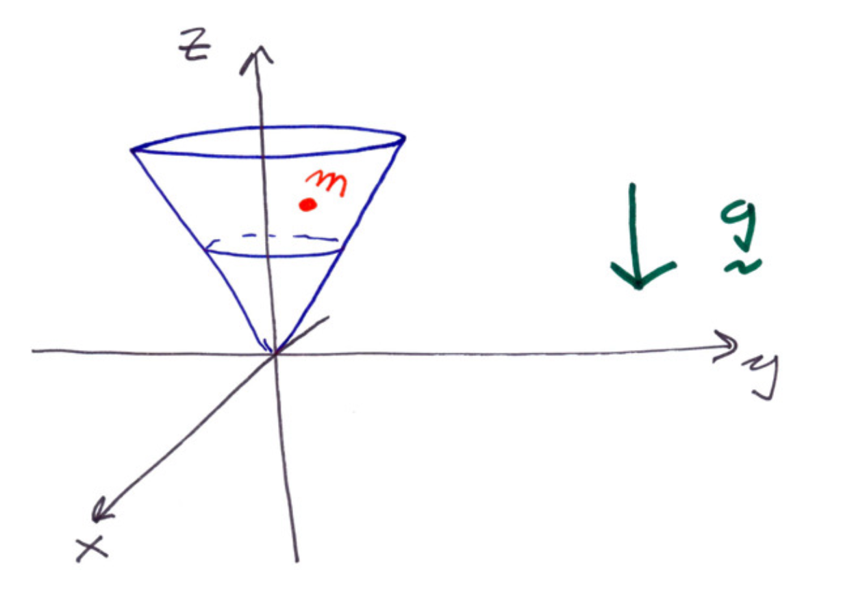
The cone is given by:
%22%2F%3E%3Cuse%20xlink%3Ahref%3D%22%23b%22%20class%3D%22typst-text%22%20transform%3D%22matrix(1%200%200%20-1%2021.592%2025.306)%22%2F%3E%3Cg%20class%3D%22typst-group%22%3E%3Cuse%20xlink%3Ahref%3D%22%23c%22%20class%3D%22typst-text%22%20transform%3D%22matrix(1%200%200%20-1%2037.428%2023.47)%22%2F%3E%3Cpath%20fill%3D%22none%22%20stroke%3D%22%23000%22%20stroke-width%3D%22.72%22%20d%3D%22M52.428%2011.08h48.316%22%20class%3D%22typst-shape%22%2F%3E%3Cuse%20xlink%3Ahref%3D%22%23d%22%20class%3D%22typst-text%22%20transform%3D%22matrix(1%200%200%20-1%2052.428%2025.306)%22%2F%3E%3Cuse%20xlink%3Ahref%3D%22%23e%22%20class%3D%22typst-text%22%20transform%3D%22matrix(1%200%200%20-1%2061.008%2020.971)%22%2F%3E%3Cuse%20xlink%3Ahref%3D%22%23f%22%20class%3D%22typst-text%22%20transform%3D%22matrix(1%200%200%20-1%2071.156%2025.306)%22%2F%3E%3Cuse%20xlink%3Ahref%3D%22%23g%22%20class%3D%22typst-text%22%20transform%3D%22matrix(1%200%200%20-1%2086.16%2025.306)%22%2F%3E%3Cuse%20xlink%3Ahref%3D%22%23e%22%20class%3D%22typst-text%22%20transform%3D%22matrix(1%200%200%20-1%2093.93%2020.971)%22%2F%3E%3C%2Fg%3E%3C%2Fg%3E%3C%2Fg%3E%3Cdefs%3E%3Csymbol%20id%3D%22a%22%20overflow%3D%22visible%22%3E%3Cpath%20d%3D%22m2.43%201.38-.255-.03c.72.705%201.275%201.215%201.65%201.56l1.44%201.335c.345.315.705.705%201.05%201.14.465.57.69.915.69%201.035%200%20.135-.075.21-.225.21-.105%200-.195-.06-.27-.195-.375-.615-.72-.915-1.05-.915s-.57.27-.705.45c-.36.435-.72.66-1.065.66-.39%200-.795-.18-1.215-.57q-.63-.585-.63-1.17c0-.15.075-.225.24-.225.105%200%20.195.075.255.21.165.435.57.645%201.185.645.21%200%20.51-.075.915-.21.36-.135.705-.21%201.02-.225a47%2047%200%200%200-1.95-1.83L2.175%202.01a14%2014%200%200%201-.825-.9C.885.525.645.18.645.045s.075-.21.24-.21c.09%200%20.18.075.285.225.375.585.78.885%201.2.885.24%200%20.51-.18.81-.555s.645-.555.99-.555c.51%200%201.02.27%201.56.795q.81.788.81%201.53c0%20.135-.075.21-.24.21q-.158%200-.27-.225a1.81%201.81%200%200%200-1.71-1.2c-.36%200-1.53.435-1.89.435%22%2F%3E%3C%2Fsymbol%3E%3Csymbol%20id%3D%22b%22%20overflow%3D%22visible%22%3E%3Cpath%20d%3D%22M10.47%205.505H1.2c-.24%200-.36-.12-.36-.345s.12-.345.36-.345h9.27c.24%200%20.36.12.36.345%200%20.18-.165.345-.36.345m0-2.82H1.2c-.24%200-.36-.12-.36-.345s.12-.345.36-.345h9.27c.24%200%20.36.12.36.345a.35.35%200%200%201-.36.345%22%2F%3E%3C%2Fsymbol%3E%3Csymbol%20id%3D%22c%22%20overflow%3D%22visible%22%3E%3Cpath%20d%3D%22M15.195%2012.105c.075.15.105.24.105.285q0%20.36-.36.36c-.15%200-.27-.105-.375-.33L6.945-3.495%203.795%203.84%201.62%202.16l.3-.33%201.05.795L6.345-5.25c.465%200%20.57.015.705.33Z%22%2F%3E%3C%2Fsymbol%3E%3Csymbol%20id%3D%22d%22%20overflow%3D%22visible%22%3E%3Cpath%20d%3D%22M7.905%205.595c0%20.69-.675%201.035-1.425%201.035-.645%200-1.155-.345-1.545-1.035-.315.69-.84%201.035-1.605%201.035-.735%200-1.335-.345-1.815-1.02C1.11%205.025.9%204.59.9%204.305c0-.135.075-.21.225-.21.135%200%20.225.075.255.21.285.87.915%201.89%201.92%201.89.495%200%20.735-.315.735-.93%200-.315-.27-1.485-.795-3.495C2.985.765%202.535.27%201.89.27c-.21%200-.405.045-.57.12q.585.225.585.81c0%20.39-.195.585-.6.585-.495%200-.87-.42-.87-.915%200-.69.705-1.035%201.44-1.035.63%200%201.14.345%201.545%201.035.285-.69.825-1.035%201.605-1.035.72%200%201.32.345%201.8%201.02.405.585.615%201.02.615%201.305%200%20.135-.075.21-.225.21-.135%200-.21-.075-.255-.21C6.705%201.305%206.03.27%205.055.27c-.495%200-.75.3-.75.915%200%20.195.075.615.24%201.29l.51%202.025c.285%201.125.75%201.695%201.41%201.695.21%200%20.405-.045.57-.12-.405-.135-.6-.405-.6-.81%200-.39.21-.585.615-.585.48%200%20.855.435.855.915%22%2F%3E%3C%2Fsymbol%3E%3Csymbol%20id%3D%22e%22%20overflow%3D%22visible%22%3E%3Cpath%20d%3D%22M1.25%204.452c.335%200%20.587.252.587.588%200%20.378-.199.577-.587.588.23.494.756.892%201.438.892.924%200%201.533-.692%201.533-1.616%200-.505-.178-.988-.546-1.46a5%205%200%200%200-.41-.504L.777.473C.64.347.661.315.661%200h4.326l.326%201.974h-.441c-.074-.556-.157-.882-.252-.955-.053-.032-.378-.053-.997-.053H1.837c.704.62%201.355%201.176%201.974%201.67.473.367.809.692%201.019.976q.473.614.473%201.292c0%20.65-.252%201.165-.767%201.543-.451.346-1.018.525-1.69.525a2.36%202.36%200%200%201-1.502-.504c-.452-.367-.683-.83-.683-1.396%200-.357.263-.62.589-.62%22%2F%3E%3C%2Fsymbol%3E%3Csymbol%20id%3D%22f%22%20overflow%3D%22visible%22%3E%3Cpath%20d%3D%22M10.47%204.11H6.195v4.275q0%20.36-.36.36t-.36-.36V4.11H1.2q-.36%200-.36-.36t.36-.36h4.275V-.885q0-.36.36-.36t.36.36V3.39h4.275q.36%200%20.36.36c0%20.195-.165.36-.36.36%22%2F%3E%3C%2Fsymbol%3E%3Csymbol%20id%3D%22g%22%20overflow%3D%22visible%22%3E%3Cpath%20d%3D%22M2.445%206.63Q1.432%206.63.87%205.505C.585%204.92.435%204.515.435%204.29c0-.135.075-.21.24-.21.21%200%20.225.09.285.315.345%201.185.825%201.785%201.44%201.785.195%200%20.3-.135.3-.405%200-.24-.075-.585-.24-1.02-.57-1.545-.855-2.58-.855-3.135%200-1.14.705-1.815%201.86-1.815.495%200%20.96.18%201.38.54q-.788-2.97-2.475-2.97-.765%200-1.035.495.9.045.9.855c0%20.375-.195.57-.6.57-.555%200-.885-.465-.885-1.02%200-.825.75-1.35%201.62-1.35%201.725%200%203.135%201.59%203.51%203.06l1.41%205.67c.045.165.06.285.06.36%200%20.3-.165.45-.48.45-.24%200-.435-.12-.57-.345-.09-.315-.165-.585-.21-.81l-.96-3.855C4.98.915%204.185.24%203.51.24c-.57%200-.855.375-.855%201.14%200%20.63.255%201.59.75%202.88.195.525.3.885.3%201.095%200%20.735-.525%201.275-1.26%201.275%22%2F%3E%3C%2Fsymbol%3E%3C%2Fdefs%3E%3C%2Fsvg%3E)
The mass of the particle is ,
the cone is smooth.
Consider the following generalized coordinates:
%22%2F%3E%3Cuse%20xlink%3Ahref%3D%22%23b%22%20class%3D%22typst-text%22%20transform%3D%22matrix(1%200%200%20-1%2021.592%2023.08)%22%2F%3E%3Cuse%20xlink%3Ahref%3D%22%23a%22%20class%3D%22typst-text%22%20transform%3D%22matrix(1%200%200%20-1%2037.428%2023.08)%22%2F%3E%3C%2Fg%3E%3C%2Fg%3E%3C%2Fg%3E%3C%2Fg%3E%3C%2Fg%3E%3Cdefs%3E%3Csymbol%20id%3D%22a%22%20overflow%3D%22visible%22%3E%3Cpath%20d%3D%22m2.43%201.38-.255-.03c.72.705%201.275%201.215%201.65%201.56l1.44%201.335c.345.315.705.705%201.05%201.14.465.57.69.915.69%201.035%200%20.135-.075.21-.225.21-.105%200-.195-.06-.27-.195-.375-.615-.72-.915-1.05-.915s-.57.27-.705.45c-.36.435-.72.66-1.065.66-.39%200-.795-.18-1.215-.57q-.63-.585-.63-1.17c0-.15.075-.225.24-.225.105%200%20.195.075.255.21.165.435.57.645%201.185.645.21%200%20.51-.075.915-.21.36-.135.705-.21%201.02-.225a47%2047%200%200%200-1.95-1.83L2.175%202.01a14%2014%200%200%201-.825-.9C.885.525.645.18.645.045s.075-.21.24-.21c.09%200%20.18.075.285.225.375.585.78.885%201.2.885.24%200%20.51-.18.81-.555s.645-.555.99-.555c.51%200%201.02.27%201.56.795q.81.788.81%201.53c0%20.135-.075.21-.24.21q-.158%200-.27-.225a1.81%201.81%200%200%200-1.71-1.2c-.36%200-1.53.435-1.89.435%22%2F%3E%3C%2Fsymbol%3E%3Csymbol%20id%3D%22b%22%20overflow%3D%22visible%22%3E%3Cpath%20d%3D%22M10.47%205.505H1.2c-.24%200-.36-.12-.36-.345s.12-.345.36-.345h9.27c.24%200%20.36.12.36.345%200%20.18-.165.345-.36.345m0-2.82H1.2c-.24%200-.36-.12-.36-.345s.12-.345.36-.345h9.27c.24%200%20.36.12.36.345a.35.35%200%200%201-.36.345%22%2F%3E%3C%2Fsymbol%3E%3C%2Fdefs%3E%3C%2Fsvg%3E)
And %22%2F%3E%3C%2Fg%3E%3C%2Fg%3E%3Cdefs%3E%3Csymbol%20id%3D%22a%22%20overflow%3D%22visible%22%3E%3Cpath%20d%3D%22M7.545%206.63c-.255%200-.48-.045-.705-.12-.945-.315-1.605-1.245-1.98-2.1-.63-1.395-.81-1.965-1.275-3.54C2.04%201.185%201.26%201.89%201.26%203c0%201.005.705%202.46%201.2%203.03q.135.157.135.225c0%20.135-.075.21-.24.21q-.382%200-.99-1.305C.96%204.29.75%203.51.75%202.835c0-1.56%201.185-2.55%202.55-2.88l-.765-2.43a1.3%201.3%200%200%201-.09-.315c0-.315.165-.48.495-.48.285%200%20.48.15.6.435L4.05-.18c.165-.015.3-.015.435-.015%201.23%200%202.325.48%203.315%201.44q1.485%201.44%201.485%203.285c0%201.17-.615%202.1-1.74%202.1m1.2-2.43c0-.945-.45-1.77-1.365-2.475C6.525%201.095%205.61.78%204.62.78c-.09%200-.18%200-.255.015-.09%200-.135%200-.135-.015.225%201.185.36%201.89.42%202.1.345%201.185%201.365%202.775%202.745%202.775.84%200%201.35-.6%201.35-1.455%22%2F%3E%3C%2Fsymbol%3E%3C%2Fdefs%3E%3C%2Fsvg%3E) be the angle of the projection of the particle on the
be the angle of the projection of the particle on the %22%2F%3E%3Cuse%20xlink%3Ahref%3D%22%23b%22%20class%3D%22typst-text%22%20transform%3D%22matrix(1%200%200%20-1%209.58%207.63)%22%2F%3E%3C%2Fg%3E%3C%2Fg%3E%3Cdefs%3E%3Csymbol%20id%3D%22a%22%20overflow%3D%22visible%22%3E%3Cpath%20d%3D%22M7.905%205.595c0%20.69-.675%201.035-1.425%201.035-.645%200-1.155-.345-1.545-1.035-.315.69-.84%201.035-1.605%201.035-.735%200-1.335-.345-1.815-1.02C1.11%205.025.9%204.59.9%204.305c0-.135.075-.21.225-.21.135%200%20.225.075.255.21.285.87.915%201.89%201.92%201.89.495%200%20.735-.315.735-.93%200-.315-.27-1.485-.795-3.495C2.985.765%202.535.27%201.89.27c-.21%200-.405.045-.57.12q.585.225.585.81c0%20.39-.195.585-.6.585-.495%200-.87-.42-.87-.915%200-.69.705-1.035%201.44-1.035.63%200%201.14.345%201.545%201.035.285-.69.825-1.035%201.605-1.035.72%200%201.32.345%201.8%201.02.405.585.615%201.02.615%201.305%200%20.135-.075.21-.225.21-.135%200-.21-.075-.255-.21C6.705%201.305%206.03.27%205.055.27c-.495%200-.75.3-.75.915%200%20.195.075.615.24%201.29l.51%202.025c.285%201.125.75%201.695%201.41%201.695.21%200%20.405-.045.57-.12-.405-.135-.6-.405-.6-.81%200-.39.21-.585.615-.585.48%200%20.855.435.855.915%22%2F%3E%3C%2Fsymbol%3E%3Csymbol%20id%3D%22b%22%20overflow%3D%22visible%22%3E%3Cpath%20d%3D%22M2.445%206.63Q1.432%206.63.87%205.505C.585%204.92.435%204.515.435%204.29c0-.135.075-.21.24-.21.21%200%20.225.09.285.315.345%201.185.825%201.785%201.44%201.785.195%200%20.3-.135.3-.405%200-.24-.075-.585-.24-1.02-.57-1.545-.855-2.58-.855-3.135%200-1.14.705-1.815%201.86-1.815.495%200%20.96.18%201.38.54q-.788-2.97-2.475-2.97-.765%200-1.035.495.9.045.9.855c0%20.375-.195.57-.6.57-.555%200-.885-.465-.885-1.02%200-.825.75-1.35%201.62-1.35%201.725%200%203.135%201.59%203.51%203.06l1.41%205.67c.045.165.06.285.06.36%200%20.3-.165.45-.48.45-.24%200-.435-.12-.57-.345-.09-.315-.165-.585-.21-.81l-.96-3.855C4.98.915%204.185.24%203.51.24c-.57%200-.855.375-.855%201.14%200%20.63.255%201.59.75%202.88.195.525.3.885.3%201.095%200%20.735-.525%201.275-1.26%201.275%22%2F%3E%3C%2Fsymbol%3E%3C%2Fdefs%3E%3C%2Fsvg%3E) plane with the axis.
plane with the axis.
Then,

The kinetic energy of the particle is given by:

The potential energy of the particle is given by:
%22%2F%3E%3Cuse%20xlink%3Ahref%3D%22%23b%22%20class%3D%22typst-text%22%20transform%3D%22matrix(1%200%200%20-1%2025.987%2020.245)%22%2F%3E%3Cuse%20xlink%3Ahref%3D%22%23c%22%20class%3D%22typst-text%22%20transform%3D%22matrix(1%200%200%20-1%2041.823%2020.245)%22%2F%3E%3Cuse%20xlink%3Ahref%3D%22%23d%22%20class%3D%22typst-text%22%20transform%3D%22matrix(1%200%200%20-1%2054.993%2020.245)%22%2F%3E%3Cuse%20xlink%3Ahref%3D%22%23e%22%20class%3D%22typst-text%22%20transform%3D%22matrix(1%200%200%20-1%2062.523%2020.245)%22%2F%3E%3C%2Fg%3E%3C%2Fg%3E%3Cdefs%3E%3Csymbol%20id%3D%22a%22%20overflow%3D%22visible%22%3E%3Cpath%20d%3D%22M9.63%2010.2c-.285%200-1.245.045-1.53.045-.225%200-.33-.12-.33-.36q0-.202.315-.225c.645%200%20.96-.195.96-.585%200-.09-.015-.195-.045-.3L7.665%203.48A4.73%204.73%200%200%200%206.36%201.26C5.655.585%204.875.255%204.035.255c-1.11%200-1.755.75-1.755%201.86l.015.135c0%20.285.045.615.15%201.005l1.44%205.775q.112.472.405.585c.09.03.345.045.78.045.39%200%20.555%200%20.555.36%200%20.15-.09.225-.255.225L3.465%2010.2l-1.905.045c-.24%200-.345-.135-.345-.36%200-.105.045-.18.12-.195.15-.015.27-.03.345-.03.465-.015.735-.045.81-.06s.105-.06.105-.135c0-.03-.015-.135-.06-.3L1.11%203.45a3.4%203.4%200%200%201-.105-.87c0-1.725%201.245-2.91%202.97-2.91.975%200%201.875.375%202.7%201.14.795.72%201.305%201.56%201.545%202.535L9.54%208.61c.195.765.615%201.035%201.545%201.05q.315.023.315.36v.06c-.045.105-.12.165-.255.165-.285%200-1.23-.045-1.515-.045%22%2F%3E%3C%2Fsymbol%3E%3Csymbol%20id%3D%22b%22%20overflow%3D%22visible%22%3E%3Cpath%20d%3D%22M10.47%205.505H1.2c-.24%200-.36-.12-.36-.345s.12-.345.36-.345h9.27c.24%200%20.36.12.36.345%200%20.18-.165.345-.36.345m0-2.82H1.2c-.24%200-.36-.12-.36-.345s.12-.345.36-.345h9.27c.24%200%20.36.12.36.345a.35.35%200%200%201-.36.345%22%2F%3E%3C%2Fsymbol%3E%3Csymbol%20id%3D%22c%22%20overflow%3D%22visible%22%3E%3Cpath%20d%3D%22M9.855%206.63c-.915%200-1.71-.45-2.385-1.335-.135.885-.705%201.335-1.725%201.335-.885%200-1.65-.39-2.28-1.185-.12.66-.645%201.185-1.41%201.185-.615%200-1.065-.495-1.38-1.47-.165-.48-.24-.765-.24-.855%200-.135.075-.21.24-.21a.27.27%200%200%201%20.165.045c.075.135.12.24.15.345.27%201.14.615%201.71%201.02%201.71q.405%200%20.405-.63c0-.195-.075-.6-.24-1.215L1.32.945c-.06-.18-.135-.57-.135-.66%200-.3.165-.45.48-.45.3%200%20.51.15.615.45.015.075.12.45.285%201.095l.315%201.335.45%201.71c.165.345.42.69.75%201.05q.652.72%201.62.72c.495%200%20.735-.33.735-.975q0-.292-.225-1.215l-.405-1.71C5.7%201.86%205.46.96%205.34.48%205.325.375%205.31.315%205.31.285q0-.45.495-.45c.165%200%20.285.045.39.15.225.225.24.33.33.735l.885%203.555c.045.195.255.54.615%201.02.45.6%201.05.9%201.785.9.495%200%20.735-.33.735-.975%200-.585-.3-1.68-.915-3.285-.135-.345-.195-.63-.195-.825%200-.735.555-1.275%201.275-1.275.675%200%201.185.375%201.56%201.125.3.6.45%201.005.45%201.2%200%20.135-.075.21-.24.21-.105-.015-.21-.15-.285-.315C11.865.87%2011.385.27%2010.74.27c-.195%200-.3.15-.3.435%200%20.225.09.555.27%201.02.615%201.605.915%202.7.915%203.27%200%201.065-.705%201.635-1.77%201.635%22%2F%3E%3C%2Fsymbol%3E%3Csymbol%20id%3D%22d%22%20overflow%3D%22visible%22%3E%3Cpath%20d%3D%22M.225-2.115c0-.645.675-.96%202.025-.96a3.8%203.8%200%200%201%201.95.525c.66.39%201.065.915%201.23%201.56l1.635%206.585c.03.15.045.24.045.285%200%20.3-.165.45-.48.45-.33%200-.54-.18-.645-.525-.33.555-.78.825-1.335.825-.96%200-1.815-.48-2.55-1.44-.675-.9-1.02-1.845-1.02-2.82%200-1.305.765-2.415%202.025-2.415.585%200%201.125.255%201.62.75l-.45-1.77C3.84-2.1%203.165-2.625%202.22-2.625q-.585%200-.99.09c.315.165.465.42.465.765%200%20.375-.21.57-.615.57-.48%200-.855-.435-.855-.915M5.34%205.88c.3-.315.45-.615.45-.915a1.3%201.3%200%200%200-.045-.195L5.04%201.935C4.95%201.59%204.695%201.23%204.29.9S3.495.405%203.15.405q-.9%200-.9%201.305c0%20.825.51%202.655.81%203.195.465.855.99%201.275%201.605%201.275.27%200%20.495-.105.675-.3%22%2F%3E%3C%2Fsymbol%3E%3Csymbol%20id%3D%22e%22%20overflow%3D%22visible%22%3E%3Cpath%20d%3D%22m2.43%201.38-.255-.03c.72.705%201.275%201.215%201.65%201.56l1.44%201.335c.345.315.705.705%201.05%201.14.465.57.69.915.69%201.035%200%20.135-.075.21-.225.21-.105%200-.195-.06-.27-.195-.375-.615-.72-.915-1.05-.915s-.57.27-.705.45c-.36.435-.72.66-1.065.66-.39%200-.795-.18-1.215-.57q-.63-.585-.63-1.17c0-.15.075-.225.24-.225.105%200%20.195.075.255.21.165.435.57.645%201.185.645.21%200%20.51-.075.915-.21.36-.135.705-.21%201.02-.225a47%2047%200%200%200-1.95-1.83L2.175%202.01a14%2014%200%200%201-.825-.9C.885.525.645.18.645.045s.075-.21.24-.21c.09%200%20.18.075.285.225.375.585.78.885%201.2.885.24%200%20.51-.18.81-.555s.645-.555.99-.555c.51%200%201.02.27%201.56.795q.81.788.81%201.53c0%20.135-.075.21-.24.21q-.158%200-.27-.225a1.81%201.81%200%200%200-1.71-1.2c-.36%200-1.53.435-1.89.435%22%2F%3E%3C%2Fsymbol%3E%3C%2Fdefs%3E%3C%2Fsvg%3E)
Thus, the Lagrangian of the particle is given by:

The momentum of the particle is given by:

Thus,

The Hamiltonian of the particle is given by:

As the Hamiltonian does not depend on the generalized coordinate ,
the generalized coordinate is a cyclical coordinate.
And the momentum %22%2F%3E%3Cuse%20xlink%3Ahref%3D%22%23b%22%20class%3D%22typst-text%22%20transform%3D%22matrix(1%200%200%20-1%208.545%2011.335)%22%2F%3E%3C%2Fg%3E%3C%2Fg%3E%3Cdefs%3E%3Csymbol%20id%3D%22a%22%20overflow%3D%22visible%22%3E%3Cpath%20d%3D%22M5.325%206.63c-.66%200-1.29-.345-1.905-1.035-.165.69-.63%201.035-1.365%201.035-.615%200-1.065-.495-1.38-1.47-.15-.495-.225-.78-.225-.87%200-.135.075-.21.24-.21a.27.27%200%200%201%20.165.045c.075.135.12.24.135.345.27%201.14.615%201.71%201.02%201.71.27%200%20.405-.21.405-.615%200-.225-.03-.48-.105-.75L.66-1.77c-.135-.495-.15-.555-.735-.555-.27%200-.405-.12-.405-.345%200-.165.09-.24.255-.24.225%200%201.005.045%201.23.045.285%200%201.185-.045%201.47-.045.225%200%20.33.12.33.36%200%20.15-.135.225-.42.225-.27%200-.675-.015-.675.165%200%20.195.615%202.55.675%202.805.3-.555.75-.84%201.35-.84.975%200%201.83.495%202.58%201.5.69.915%201.035%201.89%201.035%202.895%200%201.305-.78%202.43-2.025%202.43m-.045-.45c.585%200%20.885-.45.885-1.335%200-.405-.09-.945-.255-1.62C5.565%201.92%205.13%201.065%204.605.63%204.29.375%204.005.24%203.72.24c-.435%200-.735.195-.9.6-.135.315-.21.54-.21.66l.765%203.135c.075.33.345.675.765%201.02s.795.525%201.14.525%22%2F%3E%3C%2Fsymbol%3E%3Csymbol%20id%3D%22b%22%20overflow%3D%22visible%22%3E%3Cpath%20d%3D%22M5.901%204.63c-1.113%200-1.953-.882-2.52-2.635l-.42-1.27C2.09.84%201.165%201.26%201.165%202.12l.042.315c.074.609.515%201.386.851%201.764q.095.11.095.157c0%20.116-.063.168-.2.168-.116%200-.231-.084-.368-.241-.367-.441-.86-1.501-.86-2.268C.725.861%201.68.21%202.72-.031q-.568-1.764-.568-1.859c0-.252.137-.378.4-.378q.299%200%20.44.252c.053.105.179.735.368%201.89h.315c.903%200%201.722.305%202.457.903q1.166.96%201.166%202.3c0%20.892-.526%201.553-1.397%201.553m.945-1.763c0-.662-.357-1.208-1.082-1.638A3.7%203.7%200%200%200%203.792.66h-.284q.158.883.252%201.198c.115.398.294.756.525%201.081.452.599.945.903%201.502.903.609%200%201.06-.368%201.06-.977%22%2F%3E%3C%2Fsymbol%3E%3C%2Fdefs%3E%3C%2Fsvg%3E) is a constant.
is a constant.
Thus,

For %22%2F%3E%3C%2Fg%3E%3C%2Fg%3E%3Cdefs%3E%3Csymbol%20id%3D%22a%22%20overflow%3D%22visible%22%3E%3Cpath%20d%3D%22m2.43%201.38-.255-.03c.72.705%201.275%201.215%201.65%201.56l1.44%201.335c.345.315.705.705%201.05%201.14.465.57.69.915.69%201.035%200%20.135-.075.21-.225.21-.105%200-.195-.06-.27-.195-.375-.615-.72-.915-1.05-.915s-.57.27-.705.45c-.36.435-.72.66-1.065.66-.39%200-.795-.18-1.215-.57q-.63-.585-.63-1.17c0-.15.075-.225.24-.225.105%200%20.195.075.255.21.165.435.57.645%201.185.645.21%200%20.51-.075.915-.21.36-.135.705-.21%201.02-.225a47%2047%200%200%200-1.95-1.83L2.175%202.01a14%2014%200%200%201-.825-.9C.885.525.645.18.645.045s.075-.21.24-.21c.09%200%20.18.075.285.225.375.585.78.885%201.2.885.24%200%20.51-.18.81-.555s.645-.555.99-.555c.51%200%201.02.27%201.56.795q.81.788.81%201.53c0%20.135-.075.21-.24.21q-.158%200-.27-.225a1.81%201.81%200%200%200-1.71-1.2c-.36%200-1.53.435-1.89.435%22%2F%3E%3C%2Fsymbol%3E%3C%2Fdefs%3E%3C%2Fsvg%3E) coordinate,
coordinate,

If we are given the initial energy of the particle ,
then the Hamiltonian of the particle is given by:

Which became a first order separable ODE in .
If %22%2F%3E%3Cuse%20xlink%3Ahref%3D%22%23b%22%20class%3D%22typst-text%22%20transform%3D%22matrix(1%200%200%20-1%208.545%2014.695)%22%2F%3E%3Cuse%20xlink%3Ahref%3D%22%23c%22%20class%3D%22typst-text%22%20transform%3D%22matrix(1%200%200%20-1%2021.437%2010.99)%22%2F%3E%3Cuse%20xlink%3Ahref%3D%22%23d%22%20class%3D%22typst-text%22%20transform%3D%22matrix(1%200%200%20-1%2037.274%2010.99)%22%2F%3E%3C%2Fg%3E%3C%2Fg%3E%3Cdefs%3E%3Csymbol%20id%3D%22a%22%20overflow%3D%22visible%22%3E%3Cpath%20d%3D%22M5.325%206.63c-.66%200-1.29-.345-1.905-1.035-.165.69-.63%201.035-1.365%201.035-.615%200-1.065-.495-1.38-1.47-.15-.495-.225-.78-.225-.87%200-.135.075-.21.24-.21a.27.27%200%200%201%20.165.045c.075.135.12.24.135.345.27%201.14.615%201.71%201.02%201.71.27%200%20.405-.21.405-.615%200-.225-.03-.48-.105-.75L.66-1.77c-.135-.495-.15-.555-.735-.555-.27%200-.405-.12-.405-.345%200-.165.09-.24.255-.24.225%200%201.005.045%201.23.045.285%200%201.185-.045%201.47-.045.225%200%20.33.12.33.36%200%20.15-.135.225-.42.225-.27%200-.675-.015-.675.165%200%20.195.615%202.55.675%202.805.3-.555.75-.84%201.35-.84.975%200%201.83.495%202.58%201.5.69.915%201.035%201.89%201.035%202.895%200%201.305-.78%202.43-2.025%202.43m-.045-.45c.585%200%20.885-.45.885-1.335%200-.405-.09-.945-.255-1.62C5.565%201.92%205.13%201.065%204.605.63%204.29.375%204.005.24%203.72.24c-.435%200-.735.195-.9.6-.135.315-.21.54-.21.66l.765%203.135c.075.33.345.675.765%201.02s.795.525%201.14.525%22%2F%3E%3C%2Fsymbol%3E%3Csymbol%20id%3D%22b%22%20overflow%3D%22visible%22%3E%3Cpath%20d%3D%22M5.901%204.63c-1.113%200-1.953-.882-2.52-2.635l-.42-1.27C2.09.84%201.165%201.26%201.165%202.12l.042.315c.074.609.515%201.386.851%201.764q.095.11.095.157c0%20.116-.063.168-.2.168-.116%200-.231-.084-.368-.241-.367-.441-.86-1.501-.86-2.268C.725.861%201.68.21%202.72-.031q-.568-1.764-.568-1.859c0-.252.137-.378.4-.378q.299%200%20.44.252c.053.105.179.735.368%201.89h.315c.903%200%201.722.305%202.457.903q1.166.96%201.166%202.3c0%20.892-.526%201.553-1.397%201.553m.945-1.763c0-.662-.357-1.208-1.082-1.638A3.7%203.7%200%200%200%203.792.66h-.284q.158.883.252%201.198c.115.398.294.756.525%201.081.452.599.945.903%201.502.903.609%200%201.06-.368%201.06-.977%22%2F%3E%3C%2Fsymbol%3E%3Csymbol%20id%3D%22c%22%20overflow%3D%22visible%22%3E%3Cpath%20d%3D%22M10.47%205.505H1.2c-.24%200-.36-.12-.36-.345s.12-.345.36-.345h9.27c.24%200%20.36.12.36.345%200%20.18-.165.345-.36.345m0-2.82H1.2c-.24%200-.36-.12-.36-.345s.12-.345.36-.345h9.27c.24%200%20.36.12.36.345a.35.35%200%200%201-.36.345%22%2F%3E%3C%2Fsymbol%3E%3Csymbol%20id%3D%22d%22%20overflow%3D%22visible%22%3E%3Cpath%20d%3D%22M3.735-.33C5.85-.33%206.9%201.38%206.9%204.8c0%202.295-.48%203.825-1.425%204.575-.525.405-1.11.615-1.725.615C1.635%209.99.585%208.265.585%204.8c0-2.76.735-5.13%203.15-5.13m1.68%208.19c.105-.525.15-1.485.15-2.88%200-1.38-.06-2.4-.165-3.06Q5.107.12%203.735.12c-.345%200-.69.135-1.005.39-.405.345-.645%201.05-.75%202.13-.045.375-.06%201.155-.06%202.34%200%201.305.045%202.22.12%202.715.135.825.405%201.35.825%201.575.33.18.615.27.87.27.975%200%201.515-.795%201.68-1.68%22%2F%3E%3C%2Fsymbol%3E%3C%2Fdefs%3E%3C%2Fsvg%3E) , then the particle is moving vertically just like sliding on a smooth surface.
, then the particle is moving vertically just like sliding on a smooth surface.
If %22%2F%3E%3Cuse%20xlink%3Ahref%3D%22%23b%22%20class%3D%22typst-text%22%20transform%3D%22matrix(1%200%200%20-1%208.545%2015.655)%22%2F%3E%3Cuse%20xlink%3Ahref%3D%22%23c%22%20class%3D%22typst-text%22%20transform%3D%22matrix(1%200%200%20-1%2021.437%2011.95)%22%2F%3E%3Cuse%20xlink%3Ahref%3D%22%23d%22%20class%3D%22typst-text%22%20transform%3D%22matrix(1%200%200%20-1%2037.274%2011.95)%22%2F%3E%3C%2Fg%3E%3C%2Fg%3E%3Cdefs%3E%3Csymbol%20id%3D%22a%22%20overflow%3D%22visible%22%3E%3Cpath%20d%3D%22M5.325%206.63c-.66%200-1.29-.345-1.905-1.035-.165.69-.63%201.035-1.365%201.035-.615%200-1.065-.495-1.38-1.47-.15-.495-.225-.78-.225-.87%200-.135.075-.21.24-.21a.27.27%200%200%201%20.165.045c.075.135.12.24.135.345.27%201.14.615%201.71%201.02%201.71.27%200%20.405-.21.405-.615%200-.225-.03-.48-.105-.75L.66-1.77c-.135-.495-.15-.555-.735-.555-.27%200-.405-.12-.405-.345%200-.165.09-.24.255-.24.225%200%201.005.045%201.23.045.285%200%201.185-.045%201.47-.045.225%200%20.33.12.33.36%200%20.15-.135.225-.42.225-.27%200-.675-.015-.675.165%200%20.195.615%202.55.675%202.805.3-.555.75-.84%201.35-.84.975%200%201.83.495%202.58%201.5.69.915%201.035%201.89%201.035%202.895%200%201.305-.78%202.43-2.025%202.43m-.045-.45c.585%200%20.885-.45.885-1.335%200-.405-.09-.945-.255-1.62C5.565%201.92%205.13%201.065%204.605.63%204.29.375%204.005.24%203.72.24c-.435%200-.735.195-.9.6-.135.315-.21.54-.21.66l.765%203.135c.075.33.345.675.765%201.02s.795.525%201.14.525%22%2F%3E%3C%2Fsymbol%3E%3Csymbol%20id%3D%22b%22%20overflow%3D%22visible%22%3E%3Cpath%20d%3D%22M5.901%204.63c-1.113%200-1.953-.882-2.52-2.635l-.42-1.27C2.09.84%201.165%201.26%201.165%202.12l.042.315c.074.609.515%201.386.851%201.764q.095.11.095.157c0%20.116-.063.168-.2.168-.116%200-.231-.084-.368-.241-.367-.441-.86-1.501-.86-2.268C.725.861%201.68.21%202.72-.031q-.568-1.764-.568-1.859c0-.252.137-.378.4-.378q.299%200%20.44.252c.053.105.179.735.368%201.89h.315c.903%200%201.722.305%202.457.903q1.166.96%201.166%202.3c0%20.892-.526%201.553-1.397%201.553m.945-1.763c0-.662-.357-1.208-1.082-1.638A3.7%203.7%200%200%200%203.792.66h-.284q.158.883.252%201.198c.115.398.294.756.525%201.081.452.599.945.903%201.502.903.609%200%201.06-.368%201.06-.977%22%2F%3E%3C%2Fsymbol%3E%3Csymbol%20id%3D%22c%22%20overflow%3D%22visible%22%3E%3Cpath%20d%3D%22M10.47%202.67H5.82l.78%202.16h3.87q.36%200%20.36.36t-.36.36h-3.6l1.77%204.92c.03.045.045.075.045.12q0%20.36-.36.36c-.195%200-.3-.075-.345-.24L6.105%205.55H1.2q-.36%200-.36-.36t.36-.36h4.65l-.78-2.16H1.2q-.36%200-.36-.36t.36-.36h3.6L3.015-2.97C3-3%203-3.045%203-3.09q0-.36.36-.36c.18%200%20.285.075.33.24l1.875%205.16h4.905q.36%200%20.36.36c0%20.18-.165.36-.36.36%22%2F%3E%3C%2Fsymbol%3E%3Csymbol%20id%3D%22d%22%20overflow%3D%22visible%22%3E%3Cpath%20d%3D%22M3.735-.33C5.85-.33%206.9%201.38%206.9%204.8c0%202.295-.48%203.825-1.425%204.575-.525.405-1.11.615-1.725.615C1.635%209.99.585%208.265.585%204.8c0-2.76.735-5.13%203.15-5.13m1.68%208.19c.105-.525.15-1.485.15-2.88%200-1.38-.06-2.4-.165-3.06Q5.107.12%203.735.12c-.345%200-.69.135-1.005.39-.405.345-.645%201.05-.75%202.13-.045.375-.06%201.155-.06%202.34%200%201.305.045%202.22.12%202.715.135.825.405%201.35.825%201.575.33.18.615.27.87.27.975%200%201.515-.795%201.68-1.68%22%2F%3E%3C%2Fsymbol%3E%3C%2Fdefs%3E%3C%2Fsvg%3E) , then the term
, then the term %22%2F%3E%3Cuse%20xlink%3Ahref%3D%22%23b%22%20class%3D%22typst-text%22%20transform%3D%22matrix(1%200%200%20-1%2019.59%207.972)%22%2F%3E%3Cuse%20xlink%3Ahref%3D%22%23c%22%20class%3D%22typst-text%22%20transform%3D%22matrix(1%200%200%20-1%2019.364%2017.122)%22%2F%3E%3Cuse%20xlink%3Ahref%3D%22%23d%22%20class%3D%22typst-text%22%20transform%3D%22matrix(1%200%200%20-1%202.5%2035.59)%22%2F%3E%3Cuse%20xlink%3Ahref%3D%22%23e%22%20class%3D%22typst-text%22%20transform%3D%22matrix(1%200%200%20-1%2010%2035.59)%22%2F%3E%3Cuse%20xlink%3Ahref%3D%22%23f%22%20class%3D%22typst-text%22%20transform%3D%22matrix(1%200%200%20-1%2023.17%2035.59)%22%2F%3E%3Cuse%20xlink%3Ahref%3D%22%23b%22%20class%3D%22typst-text%22%20transform%3D%22matrix(1%200%200%20-1%2030.595%2031.255)%22%2F%3E%3Cpath%20fill%3D%22none%22%20stroke%3D%22%23000%22%20stroke-width%3D%22.72%22%20d%3D%22M2.5%2021.55h34.91%22%20class%3D%22typst-shape%22%2F%3E%3Cuse%20xlink%3Ahref%3D%22%23g%22%20class%3D%22typst-text%22%20transform%3D%22matrix(1%200%200%20-1%2042.243%2025.3)%22%2F%3E%3Cuse%20xlink%3Ahref%3D%22%23e%22%20class%3D%22typst-text%22%20transform%3D%22matrix(1%200%200%20-1%2057.246%2025.3)%22%2F%3E%3Cuse%20xlink%3Ahref%3D%22%23h%22%20class%3D%22typst-text%22%20transform%3D%22matrix(1%200%200%20-1%2070.416%2025.3)%22%2F%3E%3Cuse%20xlink%3Ahref%3D%22%23f%22%20class%3D%22typst-text%22%20transform%3D%22matrix(1%200%200%20-1%2077.946%2025.3)%22%2F%3E%3C%2Fg%3E%3C%2Fg%3E%3Cdefs%3E%3Csymbol%20id%3D%22a%22%20overflow%3D%22visible%22%3E%3Cpath%20d%3D%22M5.325%206.63c-.66%200-1.29-.345-1.905-1.035-.165.69-.63%201.035-1.365%201.035-.615%200-1.065-.495-1.38-1.47-.15-.495-.225-.78-.225-.87%200-.135.075-.21.24-.21a.27.27%200%200%201%20.165.045c.075.135.12.24.135.345.27%201.14.615%201.71%201.02%201.71.27%200%20.405-.21.405-.615%200-.225-.03-.48-.105-.75L.66-1.77c-.135-.495-.15-.555-.735-.555-.27%200-.405-.12-.405-.345%200-.165.09-.24.255-.24.225%200%201.005.045%201.23.045.285%200%201.185-.045%201.47-.045.225%200%20.33.12.33.36%200%20.15-.135.225-.42.225-.27%200-.675-.015-.675.165%200%20.195.615%202.55.675%202.805.3-.555.75-.84%201.35-.84.975%200%201.83.495%202.58%201.5.69.915%201.035%201.89%201.035%202.895%200%201.305-.78%202.43-2.025%202.43m-.045-.45c.585%200%20.885-.45.885-1.335%200-.405-.09-.945-.255-1.62C5.565%201.92%205.13%201.065%204.605.63%204.29.375%204.005.24%203.72.24c-.435%200-.735.195-.9.6-.135.315-.21.54-.21.66l.765%203.135c.075.33.345.675.765%201.02s.795.525%201.14.525%22%2F%3E%3C%2Fsymbol%3E%3Csymbol%20id%3D%22b%22%20overflow%3D%22visible%22%3E%3Cpath%20d%3D%22M1.25%204.452c.335%200%20.587.252.587.588%200%20.378-.199.577-.587.588.23.494.756.892%201.438.892.924%200%201.533-.692%201.533-1.616%200-.505-.178-.988-.546-1.46a5%205%200%200%200-.41-.504L.777.473C.64.347.661.315.661%200h4.326l.326%201.974h-.441c-.074-.556-.157-.882-.252-.955-.053-.032-.378-.053-.997-.053H1.837c.704.62%201.355%201.176%201.974%201.67.473.367.809.692%201.019.976q.473.614.473%201.292c0%20.65-.252%201.165-.767%201.543-.451.346-1.018.525-1.69.525a2.36%202.36%200%200%201-1.502-.504c-.452-.367-.683-.83-.683-1.396%200-.357.263-.62.589-.62%22%2F%3E%3C%2Fsymbol%3E%3Csymbol%20id%3D%22c%22%20overflow%3D%22visible%22%3E%3Cpath%20d%3D%22M5.901%204.63c-1.113%200-1.953-.882-2.52-2.635l-.42-1.27C2.09.84%201.165%201.26%201.165%202.12l.042.315c.074.609.515%201.386.851%201.764q.095.11.095.157c0%20.116-.063.168-.2.168-.116%200-.231-.084-.368-.241-.367-.441-.86-1.501-.86-2.268C.725.861%201.68.21%202.72-.031q-.568-1.764-.568-1.859c0-.252.137-.378.4-.378q.299%200%20.44.252c.053.105.179.735.368%201.89h.315c.903%200%201.722.305%202.457.903q1.166.96%201.166%202.3c0%20.892-.526%201.553-1.397%201.553m.945-1.763c0-.662-.357-1.208-1.082-1.638A3.7%203.7%200%200%200%203.792.66h-.284q.158.883.252%201.198c.115.398.294.756.525%201.081.452.599.945.903%201.502.903.609%200%201.06-.368%201.06-.977%22%2F%3E%3C%2Fsymbol%3E%3Csymbol%20id%3D%22d%22%20overflow%3D%22visible%22%3E%3Cpath%20d%3D%22M3.555%209.99c-.765%200-1.41-.27-1.965-.81S.75%208.01.75%207.245c0-.51.375-.885.84-.885.45%200%20.825.39.825.84%200%20.495-.36.84-.84.84-.045%200-.075%200-.105-.015.285.735.945%201.38%201.89%201.38%201.23%200%201.92-1.065%201.92-2.355%200-1.005-.51-2.085-1.53-3.225L.93.645C.735.42.75.435.75%200h5.565l.435%202.7h-.495c-.12-.765-.225-1.2-.315-1.335-.075-.075-.525-.105-1.35-.105H2.085L3.54%202.685c1.02.96%202.31%201.995%202.745%202.79q.45.787.45%201.575c0%201.77-1.38%202.94-3.18%202.94%22%2F%3E%3C%2Fsymbol%3E%3Csymbol%20id%3D%22e%22%20overflow%3D%22visible%22%3E%3Cpath%20d%3D%22M9.855%206.63c-.915%200-1.71-.45-2.385-1.335-.135.885-.705%201.335-1.725%201.335-.885%200-1.65-.39-2.28-1.185-.12.66-.645%201.185-1.41%201.185-.615%200-1.065-.495-1.38-1.47-.165-.48-.24-.765-.24-.855%200-.135.075-.21.24-.21a.27.27%200%200%201%20.165.045c.075.135.12.24.15.345.27%201.14.615%201.71%201.02%201.71q.405%200%20.405-.63c0-.195-.075-.6-.24-1.215L1.32.945c-.06-.18-.135-.57-.135-.66%200-.3.165-.45.48-.45.3%200%20.51.15.615.45.015.075.12.45.285%201.095l.315%201.335.45%201.71c.165.345.42.69.75%201.05q.652.72%201.62.72c.495%200%20.735-.33.735-.975q0-.292-.225-1.215l-.405-1.71C5.7%201.86%205.46.96%205.34.48%205.325.375%205.31.315%205.31.285q0-.45.495-.45c.165%200%20.285.045.39.15.225.225.24.33.33.735l.885%203.555c.045.195.255.54.615%201.02.45.6%201.05.9%201.785.9.495%200%20.735-.33.735-.975%200-.585-.3-1.68-.915-3.285-.135-.345-.195-.63-.195-.825%200-.735.555-1.275%201.275-1.275.675%200%201.185.375%201.56%201.125.3.6.45%201.005.45%201.2%200%20.135-.075.21-.24.21-.105-.015-.21-.15-.285-.315C11.865.87%2011.385.27%2010.74.27c-.195%200-.3.15-.3.435%200%20.225.09.555.27%201.02.615%201.605.915%202.7.915%203.27%200%201.065-.705%201.635-1.77%201.635%22%2F%3E%3C%2Fsymbol%3E%3Csymbol%20id%3D%22f%22%20overflow%3D%22visible%22%3E%3Cpath%20d%3D%22m2.43%201.38-.255-.03c.72.705%201.275%201.215%201.65%201.56l1.44%201.335c.345.315.705.705%201.05%201.14.465.57.69.915.69%201.035%200%20.135-.075.21-.225.21-.105%200-.195-.06-.27-.195-.375-.615-.72-.915-1.05-.915s-.57.27-.705.45c-.36.435-.72.66-1.065.66-.39%200-.795-.18-1.215-.57q-.63-.585-.63-1.17c0-.15.075-.225.24-.225.105%200%20.195.075.255.21.165.435.57.645%201.185.645.21%200%20.51-.075.915-.21.36-.135.705-.21%201.02-.225a47%2047%200%200%200-1.95-1.83L2.175%202.01a14%2014%200%200%201-.825-.9C.885.525.645.18.645.045s.075-.21.24-.21c.09%200%20.18.075.285.225.375.585.78.885%201.2.885.24%200%20.51-.18.81-.555s.645-.555.99-.555c.51%200%201.02.27%201.56.795q.81.788.81%201.53c0%20.135-.075.21-.24.21q-.158%200-.27-.225a1.81%201.81%200%200%200-1.71-1.2c-.36%200-1.53.435-1.89.435%22%2F%3E%3C%2Fsymbol%3E%3Csymbol%20id%3D%22g%22%20overflow%3D%22visible%22%3E%3Cpath%20d%3D%22M10.47%204.11H6.195v4.275q0%20.36-.36.36t-.36-.36V4.11H1.2q-.36%200-.36-.36t.36-.36h4.275V-.885q0-.36.36-.36t.36.36V3.39h4.275q.36%200%20.36.36c0%20.195-.165.36-.36.36%22%2F%3E%3C%2Fsymbol%3E%3Csymbol%20id%3D%22h%22%20overflow%3D%22visible%22%3E%3Cpath%20d%3D%22M.225-2.115c0-.645.675-.96%202.025-.96a3.8%203.8%200%200%201%201.95.525c.66.39%201.065.915%201.23%201.56l1.635%206.585c.03.15.045.24.045.285%200%20.3-.165.45-.48.45-.33%200-.54-.18-.645-.525-.33.555-.78.825-1.335.825-.96%200-1.815-.48-2.55-1.44-.675-.9-1.02-1.845-1.02-2.82%200-1.305.765-2.415%202.025-2.415.585%200%201.125.255%201.62.75l-.45-1.77C3.84-2.1%203.165-2.625%202.22-2.625q-.585%200-.99.09c.315.165.465.42.465.765%200%20.375-.21.57-.615.57-.48%200-.855-.435-.855-.915M5.34%205.88c.3-.315.45-.615.45-.915a1.3%201.3%200%200%200-.045-.195L5.04%201.935C4.95%201.59%204.695%201.23%204.29.9S3.495.405%203.15.405q-.9%200-.9%201.305c0%20.825.51%202.655.81%203.195.465.855.99%201.275%201.605%201.275.27%200%20.495-.105.675-.3%22%2F%3E%3C%2Fsymbol%3E%3C%2Fdefs%3E%3C%2Fsvg%3E) has lowest energy at
has lowest energy at ![z_0 = \sqrt[3]{\frac{p_{\varphi}}{m^2g}}](data:image/svg+xml;utf8,%3Csvg%20xmlns%3D%22http%3A%2F%2Fwww.w3.org%2F2000%2Fsvg%22%20xmlns%3Axlink%3D%22http%3A%2F%2Fwww.w3.org%2F1999%2Fxlink%22%20width%3D%22109.66%22%20height%3D%2251.647%22%20class%3D%22typst-doc%22%20viewBox%3D%220%200%2082.245%2038.735%22%3E%3Cpath%20fill%3D%22%23fefce8%22%20d%3D%22M0%200v38.735h82.245V0Z%22%20class%3D%22typst-shape%22%2F%3E%3Cg%20class%3D%22typst-group%22%3E%3Cg%20class%3D%22typst-group%22%3E%3Cuse%20xlink%3Ahref%3D%22%23a%22%20class%3D%22typst-text%22%20transform%3D%22matrix(1%200%200%20-1%201%2023.771)%22%2F%3E%3Cuse%20xlink%3Ahref%3D%22%23b%22%20class%3D%22typst-text%22%20transform%3D%22matrix(1%200%200%20-1%207.975%2027.476)%22%2F%3E%3Cuse%20xlink%3Ahref%3D%22%23c%22%20class%3D%22typst-text%22%20transform%3D%22matrix(1%200%200%20-1%2018.956%2023.771)%22%2F%3E%3Cuse%20xlink%3Ahref%3D%22%23d%22%20class%3D%22typst-text%22%20transform%3D%22matrix(1%200%200%20-1%2038.963%2018.322)%22%2F%3E%3Cuse%20xlink%3Ahref%3D%22%23e%22%20class%3D%22typst-text%22%20transform%3D%22matrix(1%200%200%20-1%2035.73%2023.47)%22%2F%3E%3Cpath%20fill%3D%22none%22%20stroke%3D%22%23000%22%20stroke-width%3D%22.72%22%20d%3D%22M50.73%202.08h30.515%22%20class%3D%22typst-shape%22%2F%3E%3Cg%20class%3D%22typst-group%22%3E%3Cuse%20xlink%3Ahref%3D%22%23f%22%20class%3D%22typst-text%22%20transform%3D%22matrix(1%200%200%20-1%2057.852%2011.888)%22%2F%3E%3Cuse%20xlink%3Ahref%3D%22%23g%22%20class%3D%22typst-text%22%20transform%3D%22matrix(1%200%200%20-1%2065.397%2015.593)%22%2F%3E%3Cuse%20xlink%3Ahref%3D%22%23h%22%20class%3D%22typst-text%22%20transform%3D%22matrix(1%200%200%20-1%2052.23%2034.062)%22%2F%3E%3Cuse%20xlink%3Ahref%3D%22%23i%22%20class%3D%22typst-text%22%20transform%3D%22matrix(1%200%200%20-1%2065.4%2029.726)%22%2F%3E%3Cuse%20xlink%3Ahref%3D%22%23j%22%20class%3D%22typst-text%22%20transform%3D%22matrix(1%200%200%20-1%2072.215%2034.062)%22%2F%3E%3Cpath%20fill%3D%22none%22%20stroke%3D%22%23000%22%20stroke-width%3D%22.72%22%20d%3D%22M52.23%2020.021h27.515%22%20class%3D%22typst-shape%22%2F%3E%3C%2Fg%3E%3C%2Fg%3E%3C%2Fg%3E%3Cdefs%3E%3Csymbol%20id%3D%22a%22%20overflow%3D%22visible%22%3E%3Cpath%20d%3D%22m2.43%201.38-.255-.03c.72.705%201.275%201.215%201.65%201.56l1.44%201.335c.345.315.705.705%201.05%201.14.465.57.69.915.69%201.035%200%20.135-.075.21-.225.21-.105%200-.195-.06-.27-.195-.375-.615-.72-.915-1.05-.915s-.57.27-.705.45c-.36.435-.72.66-1.065.66-.39%200-.795-.18-1.215-.57q-.63-.585-.63-1.17c0-.15.075-.225.24-.225.105%200%20.195.075.255.21.165.435.57.645%201.185.645.21%200%20.51-.075.915-.21.36-.135.705-.21%201.02-.225a47%2047%200%200%200-1.95-1.83L2.175%202.01a14%2014%200%200%201-.825-.9C.885.525.645.18.645.045s.075-.21.24-.21c.09%200%20.18.075.285.225.375.585.78.885%201.2.885.24%200%20.51-.18.81-.555s.645-.555.99-.555c.51%200%201.02.27%201.56.795q.81.788.81%201.53c0%20.135-.075.21-.24.21q-.158%200-.27-.225a1.81%201.81%200%200%200-1.71-1.2c-.36%200-1.53.435-1.89.435%22%2F%3E%3C%2Fsymbol%3E%3Csymbol%20id%3D%22b%22%20overflow%3D%22visible%22%3E%3Cpath%20d%3D%22M5.418%203.35c0%201.186-.21%202.089-.62%202.709-.335.524-1.007.913-1.816.913-.336%200-.64-.053-.903-.168C.924%206.321.546%204.977.546%203.349c0-.357.021-.693.052-1.018C.778.956%201.418-.21%202.983-.21c.336%200%20.64.052.903.168C5.04.431%205.418%201.743%205.418%203.349M4.221%205.68c.115-.388.178-1.112.178-2.194%200-1.029-.042-1.754-.136-2.184C4.137.682%203.696.168%202.982.168c-.263%200-.525.084-.767.262-.325.242-.524.715-.608%201.439-.032.241-.042.777-.042%201.617%200%201.019.052%201.722.157%202.1q.268%201.008%201.26%201.008c.63%200%201.092-.41%201.239-.913%22%2F%3E%3C%2Fsymbol%3E%3Csymbol%20id%3D%22c%22%20overflow%3D%22visible%22%3E%3Cpath%20d%3D%22M10.47%205.505H1.2c-.24%200-.36-.12-.36-.345s.12-.345.36-.345h9.27c.24%200%20.36.12.36.345%200%20.18-.165.345-.36.345m0-2.82H1.2c-.24%200-.36-.12-.36-.345s.12-.345.36-.345h9.27c.24%200%20.36.12.36.345a.35.35%200%200%201-.36.345%22%2F%3E%3C%2Fsymbol%3E%3Csymbol%20id%3D%22d%22%20overflow%3D%22visible%22%3E%3Cpath%20d%3D%22M3.195%202.64q1.048.391%201.05%201.268c0%20.36-.21.645-.622.847a2.5%202.5%200%200%201-1.096.24q-.618%200-1.08-.225-.594-.293-.592-.855c0-.27.188-.473.458-.473a.45.45%200%200%201%20.45.458c0%20.232-.113.382-.33.435.224.218.585.322%201.072.322.51%200%20.893-.262.893-.75%200-.614-.443-1.087-1.028-1.124a16%2016%200%200%200-.428-.023c-.127-.007-.187-.06-.187-.15%200-.158.075-.158.233-.158h.487c.69%200%201.102-.434%201.102-1.124C3.577.63%203.172.194%202.482.194c-.592%200-1.02.112-1.275.337q.36.09.36.473a.47.47%200%200%201-.48.48C.795%201.485.6%201.282.6.99c0-.412.225-.727.683-.93q.504-.225%201.222-.225c.487%200%20.93.12%201.32.36Q4.5.623%204.5%201.32c0%20.705-.667%201.162-1.305%201.32%22%2F%3E%3C%2Fsymbol%3E%3Csymbol%20id%3D%22e%22%20overflow%3D%22visible%22%3E%3Cpath%20d%3D%22M7.005-10.995%203.81%203.9%201.785.705C1.71.6%201.665.54%201.665.495c0-.06.09-.165.285-.33l.96%201.53L6.33-14.25c.585%200%20.63-.015.735.435L15.24%2021.06c.045.18.06.285.06.33q0%20.36-.36.36c-.18%200-.3-.15-.375-.45Z%22%2F%3E%3C%2Fsymbol%3E%3Csymbol%20id%3D%22f%22%20overflow%3D%22visible%22%3E%3Cpath%20d%3D%22M5.325%206.63c-.66%200-1.29-.345-1.905-1.035-.165.69-.63%201.035-1.365%201.035-.615%200-1.065-.495-1.38-1.47-.15-.495-.225-.78-.225-.87%200-.135.075-.21.24-.21a.27.27%200%200%201%20.165.045c.075.135.12.24.135.345.27%201.14.615%201.71%201.02%201.71.27%200%20.405-.21.405-.615%200-.225-.03-.48-.105-.75L.66-1.77c-.135-.495-.15-.555-.735-.555-.27%200-.405-.12-.405-.345%200-.165.09-.24.255-.24.225%200%201.005.045%201.23.045.285%200%201.185-.045%201.47-.045.225%200%20.33.12.33.36%200%20.15-.135.225-.42.225-.27%200-.675-.015-.675.165%200%20.195.615%202.55.675%202.805.3-.555.75-.84%201.35-.84.975%200%201.83.495%202.58%201.5.69.915%201.035%201.89%201.035%202.895%200%201.305-.78%202.43-2.025%202.43m-.045-.45c.585%200%20.885-.45.885-1.335%200-.405-.09-.945-.255-1.62C5.565%201.92%205.13%201.065%204.605.63%204.29.375%204.005.24%203.72.24c-.435%200-.735.195-.9.6-.135.315-.21.54-.21.66l.765%203.135c.075.33.345.675.765%201.02s.795.525%201.14.525%22%2F%3E%3C%2Fsymbol%3E%3Csymbol%20id%3D%22g%22%20overflow%3D%22visible%22%3E%3Cpath%20d%3D%22M5.901%204.63c-1.113%200-1.953-.882-2.52-2.635l-.42-1.27C2.09.84%201.165%201.26%201.165%202.12l.042.315c.074.609.515%201.386.851%201.764q.095.11.095.157c0%20.116-.063.168-.2.168-.116%200-.231-.084-.368-.241-.367-.441-.86-1.501-.86-2.268C.725.861%201.68.21%202.72-.031q-.568-1.764-.568-1.859c0-.252.137-.378.4-.378q.299%200%20.44.252c.053.105.179.735.368%201.89h.315c.903%200%201.722.305%202.457.903q1.166.96%201.166%202.3c0%20.892-.526%201.553-1.397%201.553m.945-1.763c0-.662-.357-1.208-1.082-1.638A3.7%203.7%200%200%200%203.792.66h-.284q.158.883.252%201.198c.115.398.294.756.525%201.081.452.599.945.903%201.502.903.609%200%201.06-.368%201.06-.977%22%2F%3E%3C%2Fsymbol%3E%3Csymbol%20id%3D%22h%22%20overflow%3D%22visible%22%3E%3Cpath%20d%3D%22M9.855%206.63c-.915%200-1.71-.45-2.385-1.335-.135.885-.705%201.335-1.725%201.335-.885%200-1.65-.39-2.28-1.185-.12.66-.645%201.185-1.41%201.185-.615%200-1.065-.495-1.38-1.47-.165-.48-.24-.765-.24-.855%200-.135.075-.21.24-.21a.27.27%200%200%201%20.165.045c.075.135.12.24.15.345.27%201.14.615%201.71%201.02%201.71q.405%200%20.405-.63c0-.195-.075-.6-.24-1.215L1.32.945c-.06-.18-.135-.57-.135-.66%200-.3.165-.45.48-.45.3%200%20.51.15.615.45.015.075.12.45.285%201.095l.315%201.335.45%201.71c.165.345.42.69.75%201.05q.652.72%201.62.72c.495%200%20.735-.33.735-.975q0-.292-.225-1.215l-.405-1.71C5.7%201.86%205.46.96%205.34.48%205.325.375%205.31.315%205.31.285q0-.45.495-.45c.165%200%20.285.045.39.15.225.225.24.33.33.735l.885%203.555c.045.195.255.54.615%201.02.45.6%201.05.9%201.785.9.495%200%20.735-.33.735-.975%200-.585-.3-1.68-.915-3.285-.135-.345-.195-.63-.195-.825%200-.735.555-1.275%201.275-1.275.675%200%201.185.375%201.56%201.125.3.6.45%201.005.45%201.2%200%20.135-.075.21-.24.21-.105-.015-.21-.15-.285-.315C11.865.87%2011.385.27%2010.74.27c-.195%200-.3.15-.3.435%200%20.225.09.555.27%201.02.615%201.605.915%202.7.915%203.27%200%201.065-.705%201.635-1.77%201.635%22%2F%3E%3C%2Fsymbol%3E%3Csymbol%20id%3D%22i%22%20overflow%3D%22visible%22%3E%3Cpath%20d%3D%22M1.25%204.452c.335%200%20.587.252.587.588%200%20.378-.199.577-.587.588.23.494.756.892%201.438.892.924%200%201.533-.692%201.533-1.616%200-.505-.178-.988-.546-1.46a5%205%200%200%200-.41-.504L.777.473C.64.347.661.315.661%200h4.326l.326%201.974h-.441c-.074-.556-.157-.882-.252-.955-.053-.032-.378-.053-.997-.053H1.837c.704.62%201.355%201.176%201.974%201.67.473.367.809.692%201.019.976q.473.614.473%201.292c0%20.65-.252%201.165-.767%201.543-.451.346-1.018.525-1.69.525a2.36%202.36%200%200%201-1.502-.504c-.452-.367-.683-.83-.683-1.396%200-.357.263-.62.589-.62%22%2F%3E%3C%2Fsymbol%3E%3Csymbol%20id%3D%22j%22%20overflow%3D%22visible%22%3E%3Cpath%20d%3D%22M.225-2.115c0-.645.675-.96%202.025-.96a3.8%203.8%200%200%201%201.95.525c.66.39%201.065.915%201.23%201.56l1.635%206.585c.03.15.045.24.045.285%200%20.3-.165.45-.48.45-.33%200-.54-.18-.645-.525-.33.555-.78.825-1.335.825-.96%200-1.815-.48-2.55-1.44-.675-.9-1.02-1.845-1.02-2.82%200-1.305.765-2.415%202.025-2.415.585%200%201.125.255%201.62.75l-.45-1.77C3.84-2.1%203.165-2.625%202.22-2.625q-.585%200-.99.09c.315.165.465.42.465.765%200%20.375-.21.57-.615.57-.48%200-.855-.435-.855-.915M5.34%205.88c.3-.315.45-.615.45-.915a1.3%201.3%200%200%200-.045-.195L5.04%201.935C4.95%201.59%204.695%201.23%204.29.9S3.495.405%203.15.405q-.9%200-.9%201.305c0%20.825.51%202.655.81%203.195.465.855.99%201.275%201.605%201.275.27%200%20.495-.105.675-.3%22%2F%3E%3C%2Fsymbol%3E%3C%2Fdefs%3E%3C%2Fsvg%3E) with energy
with energy
%22%2F%3E%3Cuse%20xlink%3Ahref%3D%22%23b%22%20class%3D%22typst-text%22%20transform%3D%22matrix(1%200%200%20-1%2012.07%2014.905)%22%2F%3E%3C%2Fg%3E%3C%2Fg%3E%3Cdefs%3E%3Csymbol%20id%3D%22a%22%20overflow%3D%22visible%22%3E%3Cpath%20d%3D%22M2.985%209.84c0-.15.165-.225.48-.225.6%200%20.9-.06.9-.195%200-.045-.03-.15-.075-.345L2.34%201.23C2.265.9%202.115.705%201.89.63%201.785.6%201.515.585%201.05.585.72.585.57.555.57.24.57.075.735%200%201.05%200h7.695c.36%200%20.39.03.51.285l.6%201.35c.405.93.69%201.62.855%202.085-.03.135-.075.225-.24.225-.105%200-.195-.075-.255-.21-.375-.885-.735-1.56-1.095-2.04-.6-.81-1.485-1.11-2.895-1.11H4.05c-.15%200-.255%200-.315.015-.09%200-.135.03-.135.075%200%20.03.03.135.075.33l.99%204.005H6.09c.705%200%201.08-.09%201.155-.285a.9.9%200%200%200%20.045-.33c0-.195-.03-.435-.105-.72a.5.5%200%200%201-.045-.18c0-.15.09-.225.255-.225.135%200%20.225.12.285.345l.84%203.48c0%20.15-.075.225-.24.225-.12%200-.21-.105-.255-.315-.15-.585-.345-.96-.6-1.14s-.675-.27-1.29-.27h-1.32l.87%203.495c.12.51.12.525.75.525H8.52q1.148%200%201.575-.225.63-.338.63-1.35c0-.255-.015-.525-.06-.78%200-.03%200-.075-.015-.135V6.99c0-.165.075-.24.225-.24s.24.135.27.42l.3%202.565c.045.42-.06.465-.465.465H3.495c-.345%200-.51-.015-.51-.36%22%2F%3E%3C%2Fsymbol%3E%3Csymbol%20id%3D%22b%22%20overflow%3D%22visible%22%3E%3Cpath%20d%3D%22M5.418%203.35c0%201.186-.21%202.089-.62%202.709-.335.524-1.007.913-1.816.913-.336%200-.64-.053-.903-.168C.924%206.321.546%204.977.546%203.349c0-.357.021-.693.052-1.018C.778.956%201.418-.21%202.983-.21c.336%200%20.64.052.903.168C5.04.431%205.418%201.743%205.418%203.349M4.221%205.68c.115-.388.178-1.112.178-2.194%200-1.029-.042-1.754-.136-2.184C4.137.682%203.696.168%202.982.168c-.263%200-.525.084-.767.262-.325.242-.524.715-.608%201.439-.032.241-.042.777-.042%201.617%200%201.019.052%201.722.157%202.1q.268%201.008%201.26%201.008c.63%200%201.092-.41%201.239-.913%22%2F%3E%3C%2Fsymbol%3E%3C%2Fdefs%3E%3C%2Fsvg%3E) .
.
If %22%2F%3E%3Cuse%20xlink%3Ahref%3D%22%23b%22%20class%3D%22typst-text%22%20transform%3D%22matrix(1%200%200%20-1%2017.047%2011.2)%22%2F%3E%3Cuse%20xlink%3Ahref%3D%22%23a%22%20class%3D%22typst-text%22%20transform%3D%22matrix(1%200%200%20-1%2032.883%2011.2)%22%2F%3E%3Cuse%20xlink%3Ahref%3D%22%23c%22%20class%3D%22typst-text%22%20transform%3D%22matrix(1%200%200%20-1%2043.953%2014.905)%22%2F%3E%3C%2Fg%3E%3C%2Fg%3E%3Cdefs%3E%3Csymbol%20id%3D%22a%22%20overflow%3D%22visible%22%3E%3Cpath%20d%3D%22M2.985%209.84c0-.15.165-.225.48-.225.6%200%20.9-.06.9-.195%200-.045-.03-.15-.075-.345L2.34%201.23C2.265.9%202.115.705%201.89.63%201.785.6%201.515.585%201.05.585.72.585.57.555.57.24.57.075.735%200%201.05%200h7.695c.36%200%20.39.03.51.285l.6%201.35c.405.93.69%201.62.855%202.085-.03.135-.075.225-.24.225-.105%200-.195-.075-.255-.21-.375-.885-.735-1.56-1.095-2.04-.6-.81-1.485-1.11-2.895-1.11H4.05c-.15%200-.255%200-.315.015-.09%200-.135.03-.135.075%200%20.03.03.135.075.33l.99%204.005H6.09c.705%200%201.08-.09%201.155-.285a.9.9%200%200%200%20.045-.33c0-.195-.03-.435-.105-.72a.5.5%200%200%201-.045-.18c0-.15.09-.225.255-.225.135%200%20.225.12.285.345l.84%203.48c0%20.15-.075.225-.24.225-.12%200-.21-.105-.255-.315-.15-.585-.345-.96-.6-1.14s-.675-.27-1.29-.27h-1.32l.87%203.495c.12.51.12.525.75.525H8.52q1.148%200%201.575-.225.63-.338.63-1.35c0-.255-.015-.525-.06-.78%200-.03%200-.075-.015-.135V6.99c0-.165.075-.24.225-.24s.24.135.27.42l.3%202.565c.045.42-.06.465-.465.465H3.495c-.345%200-.51-.015-.51-.36%22%2F%3E%3C%2Fsymbol%3E%3Csymbol%20id%3D%22b%22%20overflow%3D%22visible%22%3E%3Cpath%20d%3D%22M10.47%205.505H1.2c-.24%200-.36-.12-.36-.345s.12-.345.36-.345h9.27c.24%200%20.36.12.36.345%200%20.18-.165.345-.36.345m0-2.82H1.2c-.24%200-.36-.12-.36-.345s.12-.345.36-.345h9.27c.24%200%20.36.12.36.345a.35.35%200%200%201-.36.345%22%2F%3E%3C%2Fsymbol%3E%3Csymbol%20id%3D%22c%22%20overflow%3D%22visible%22%3E%3Cpath%20d%3D%22M5.418%203.35c0%201.186-.21%202.089-.62%202.709-.335.524-1.007.913-1.816.913-.336%200-.64-.053-.903-.168C.924%206.321.546%204.977.546%203.349c0-.357.021-.693.052-1.018C.778.956%201.418-.21%202.983-.21c.336%200%20.64.052.903.168C5.04.431%205.418%201.743%205.418%203.349M4.221%205.68c.115-.388.178-1.112.178-2.194%200-1.029-.042-1.754-.136-2.184C4.137.682%203.696.168%202.982.168c-.263%200-.525.084-.767.262-.325.242-.524.715-.608%201.439-.032.241-.042.777-.042%201.617%200%201.019.052%201.722.157%202.1q.268%201.008%201.26%201.008c.63%200%201.092-.41%201.239-.913%22%2F%3E%3C%2Fsymbol%3E%3C%2Fdefs%3E%3C%2Fsvg%3E) , then
, then %22%2F%3E%3Cuse%20xlink%3Ahref%3D%22%23b%22%20class%3D%22typst-text%22%20transform%3D%22matrix(1%200%200%20-1%2023.185%2013.537)%22%2F%3E%3Cuse%20xlink%3Ahref%3D%22%23c%22%20class%3D%22typst-text%22%20transform%3D%22matrix(1%200%200%20-1%2014.17%2013.417)%22%2F%3E%3Cuse%20xlink%3Ahref%3D%22%23d%22%20class%3D%22typst-text%22%20transform%3D%22matrix(1%200%200%20-1%2021.595%207.972)%22%2F%3E%3Cuse%20xlink%3Ahref%3D%22%23e%22%20class%3D%22typst-text%22%20transform%3D%22matrix(1%200%200%20-1%2032.576%2013.417)%22%2F%3E%3Cuse%20xlink%3Ahref%3D%22%23f%22%20class%3D%22typst-text%22%20transform%3D%22matrix(1%200%200%20-1%2048.413%2013.417)%22%2F%3E%3C%2Fg%3E%3C%2Fg%3E%3Cdefs%3E%3Csymbol%20id%3D%22a%22%20overflow%3D%22visible%22%3E%3Cpath%20d%3D%22M9.855%206.63c-.915%200-1.71-.45-2.385-1.335-.135.885-.705%201.335-1.725%201.335-.885%200-1.65-.39-2.28-1.185-.12.66-.645%201.185-1.41%201.185-.615%200-1.065-.495-1.38-1.47-.165-.48-.24-.765-.24-.855%200-.135.075-.21.24-.21a.27.27%200%200%201%20.165.045c.075.135.12.24.15.345.27%201.14.615%201.71%201.02%201.71q.405%200%20.405-.63c0-.195-.075-.6-.24-1.215L1.32.945c-.06-.18-.135-.57-.135-.66%200-.3.165-.45.48-.45.3%200%20.51.15.615.45.015.075.12.45.285%201.095l.315%201.335.45%201.71c.165.345.42.69.75%201.05q.652.72%201.62.72c.495%200%20.735-.33.735-.975q0-.292-.225-1.215l-.405-1.71C5.7%201.86%205.46.96%205.34.48%205.325.375%205.31.315%205.31.285q0-.45.495-.45c.165%200%20.285.045.39.15.225.225.24.33.33.735l.885%203.555c.045.195.255.54.615%201.02.45.6%201.05.9%201.785.9.495%200%20.735-.33.735-.975%200-.585-.3-1.68-.915-3.285-.135-.345-.195-.63-.195-.825%200-.735.555-1.275%201.275-1.275.675%200%201.185.375%201.56%201.125.3.6.45%201.005.45%201.2%200%20.135-.075.21-.24.21-.105-.015-.21-.15-.285-.315C11.865.87%2011.385.27%2010.74.27c-.195%200-.3.15-.3.435%200%20.225.09.555.27%201.02.615%201.605.915%202.7.915%203.27%200%201.065-.705%201.635-1.77%201.635%22%2F%3E%3C%2Fsymbol%3E%3Csymbol%20id%3D%22b%22%20overflow%3D%22visible%22%3E%3Cpath%20d%3D%22M-3.165%209.36a.8.8%200%200%201-.795.795.813.813%200%200%201-.81-.795.8.8%200%200%201%20.795-.795c.435%200%20.81.36.81.795%22%2F%3E%3C%2Fsymbol%3E%3Csymbol%20id%3D%22c%22%20overflow%3D%22visible%22%3E%3Cpath%20d%3D%22m2.43%201.38-.255-.03c.72.705%201.275%201.215%201.65%201.56l1.44%201.335c.345.315.705.705%201.05%201.14.465.57.69.915.69%201.035%200%20.135-.075.21-.225.21-.105%200-.195-.06-.27-.195-.375-.615-.72-.915-1.05-.915s-.57.27-.705.45c-.36.435-.72.66-1.065.66-.39%200-.795-.18-1.215-.57q-.63-.585-.63-1.17c0-.15.075-.225.24-.225.105%200%20.195.075.255.21.165.435.57.645%201.185.645.21%200%20.51-.075.915-.21.36-.135.705-.21%201.02-.225a47%2047%200%200%200-1.95-1.83L2.175%202.01a14%2014%200%200%201-.825-.9C.885.525.645.18.645.045s.075-.21.24-.21c.09%200%20.18.075.285.225.375.585.78.885%201.2.885.24%200%20.51-.18.81-.555s.645-.555.99-.555c.51%200%201.02.27%201.56.795q.81.788.81%201.53c0%20.135-.075.21-.24.21q-.158%200-.27-.225a1.81%201.81%200%200%200-1.71-1.2c-.36%200-1.53.435-1.89.435%22%2F%3E%3C%2Fsymbol%3E%3Csymbol%20id%3D%22d%22%20overflow%3D%22visible%22%3E%3Cpath%20d%3D%22M1.25%204.452c.335%200%20.587.252.587.588%200%20.378-.199.577-.587.588.23.494.756.892%201.438.892.924%200%201.533-.692%201.533-1.616%200-.505-.178-.988-.546-1.46a5%205%200%200%200-.41-.504L.777.473C.64.347.661.315.661%200h4.326l.326%201.974h-.441c-.074-.556-.157-.882-.252-.955-.053-.032-.378-.053-.997-.053H1.837c.704.62%201.355%201.176%201.974%201.67.473.367.809.692%201.019.976q.473.614.473%201.292c0%20.65-.252%201.165-.767%201.543-.451.346-1.018.525-1.69.525a2.36%202.36%200%200%201-1.502-.504c-.452-.367-.683-.83-.683-1.396%200-.357.263-.62.589-.62%22%2F%3E%3C%2Fsymbol%3E%3Csymbol%20id%3D%22e%22%20overflow%3D%22visible%22%3E%3Cpath%20d%3D%22M10.47%205.505H1.2c-.24%200-.36-.12-.36-.345s.12-.345.36-.345h9.27c.24%200%20.36.12.36.345%200%20.18-.165.345-.36.345m0-2.82H1.2c-.24%200-.36-.12-.36-.345s.12-.345.36-.345h9.27c.24%200%20.36.12.36.345a.35.35%200%200%201-.36.345%22%2F%3E%3C%2Fsymbol%3E%3Csymbol%20id%3D%22f%22%20overflow%3D%22visible%22%3E%3Cpath%20d%3D%22M3.735-.33C5.85-.33%206.9%201.38%206.9%204.8c0%202.295-.48%203.825-1.425%204.575-.525.405-1.11.615-1.725.615C1.635%209.99.585%208.265.585%204.8c0-2.76.735-5.13%203.15-5.13m1.68%208.19c.105-.525.15-1.485.15-2.88%200-1.38-.06-2.4-.165-3.06Q5.107.12%203.735.12c-.345%200-.69.135-1.005.39-.405.345-.645%201.05-.75%202.13-.045.375-.06%201.155-.06%202.34%200%201.305.045%202.22.12%202.715.135.825.405%201.35.825%201.575.33.18.615.27.87.27.975%200%201.515-.795%201.68-1.68%22%2F%3E%3C%2Fsymbol%3E%3C%2Fdefs%3E%3C%2Fsvg%3E) , and the particle is doing a circular motion on the cone.
, and the particle is doing a circular motion on the cone.
If %22%2F%3E%3Cuse%20xlink%3Ahref%3D%22%23b%22%20class%3D%22typst-text%22%20transform%3D%22matrix(1%200%200%20-1%2017.047%2011.2)%22%2F%3E%3Cuse%20xlink%3Ahref%3D%22%23a%22%20class%3D%22typst-text%22%20transform%3D%22matrix(1%200%200%20-1%2032.883%2011.2)%22%2F%3E%3Cuse%20xlink%3Ahref%3D%22%23c%22%20class%3D%22typst-text%22%20transform%3D%22matrix(1%200%200%20-1%2043.953%2014.905)%22%2F%3E%3C%2Fg%3E%3C%2Fg%3E%3Cdefs%3E%3Csymbol%20id%3D%22a%22%20overflow%3D%22visible%22%3E%3Cpath%20d%3D%22M2.985%209.84c0-.15.165-.225.48-.225.6%200%20.9-.06.9-.195%200-.045-.03-.15-.075-.345L2.34%201.23C2.265.9%202.115.705%201.89.63%201.785.6%201.515.585%201.05.585.72.585.57.555.57.24.57.075.735%200%201.05%200h7.695c.36%200%20.39.03.51.285l.6%201.35c.405.93.69%201.62.855%202.085-.03.135-.075.225-.24.225-.105%200-.195-.075-.255-.21-.375-.885-.735-1.56-1.095-2.04-.6-.81-1.485-1.11-2.895-1.11H4.05c-.15%200-.255%200-.315.015-.09%200-.135.03-.135.075%200%20.03.03.135.075.33l.99%204.005H6.09c.705%200%201.08-.09%201.155-.285a.9.9%200%200%200%20.045-.33c0-.195-.03-.435-.105-.72a.5.5%200%200%201-.045-.18c0-.15.09-.225.255-.225.135%200%20.225.12.285.345l.84%203.48c0%20.15-.075.225-.24.225-.12%200-.21-.105-.255-.315-.15-.585-.345-.96-.6-1.14s-.675-.27-1.29-.27h-1.32l.87%203.495c.12.51.12.525.75.525H8.52q1.148%200%201.575-.225.63-.338.63-1.35c0-.255-.015-.525-.06-.78%200-.03%200-.075-.015-.135V6.99c0-.165.075-.24.225-.24s.24.135.27.42l.3%202.565c.045.42-.06.465-.465.465H3.495c-.345%200-.51-.015-.51-.36%22%2F%3E%3C%2Fsymbol%3E%3Csymbol%20id%3D%22b%22%20overflow%3D%22visible%22%3E%3Cpath%20d%3D%22M10.29%203.405c.15.075.225.18.225.345s-.075.27-.225.345l-8.61%204.08a.5.5%200%200%201-.165.03c-.24%200-.36-.12-.36-.375%200-.135.075-.24.21-.3l8.01-3.78-8.01-3.78c-.135-.06-.21-.165-.21-.3%200-.255.12-.375.36-.375.06%200%20.12.015.165.03Z%22%2F%3E%3C%2Fsymbol%3E%3Csymbol%20id%3D%22c%22%20overflow%3D%22visible%22%3E%3Cpath%20d%3D%22M5.418%203.35c0%201.186-.21%202.089-.62%202.709-.335.524-1.007.913-1.816.913-.336%200-.64-.053-.903-.168C.924%206.321.546%204.977.546%203.349c0-.357.021-.693.052-1.018C.778.956%201.418-.21%202.983-.21c.336%200%20.64.052.903.168C5.04.431%205.418%201.743%205.418%203.349M4.221%205.68c.115-.388.178-1.112.178-2.194%200-1.029-.042-1.754-.136-2.184C4.137.682%203.696.168%202.982.168c-.263%200-.525.084-.767.262-.325.242-.524.715-.608%201.439-.032.241-.042.777-.042%201.617%200%201.019.052%201.722.157%202.1q.268%201.008%201.26%201.008c.63%200%201.092-.41%201.239-.913%22%2F%3E%3C%2Fsymbol%3E%3C%2Fdefs%3E%3C%2Fsvg%3E) , then the particle is doing oscillatory motion on the cone.
By using Taylor expansion of around
, then the particle is doing oscillatory motion on the cone.
By using Taylor expansion of around %22%2F%3E%3Cuse%20xlink%3Ahref%3D%22%23b%22%20class%3D%22typst-text%22%20transform%3D%22matrix(1%200%200%20-1%207.975%2011.335)%22%2F%3E%3C%2Fg%3E%3C%2Fg%3E%3Cdefs%3E%3Csymbol%20id%3D%22a%22%20overflow%3D%22visible%22%3E%3Cpath%20d%3D%22m2.43%201.38-.255-.03c.72.705%201.275%201.215%201.65%201.56l1.44%201.335c.345.315.705.705%201.05%201.14.465.57.69.915.69%201.035%200%20.135-.075.21-.225.21-.105%200-.195-.06-.27-.195-.375-.615-.72-.915-1.05-.915s-.57.27-.705.45c-.36.435-.72.66-1.065.66-.39%200-.795-.18-1.215-.57q-.63-.585-.63-1.17c0-.15.075-.225.24-.225.105%200%20.195.075.255.21.165.435.57.645%201.185.645.21%200%20.51-.075.915-.21.36-.135.705-.21%201.02-.225a47%2047%200%200%200-1.95-1.83L2.175%202.01a14%2014%200%200%201-.825-.9C.885.525.645.18.645.045s.075-.21.24-.21c.09%200%20.18.075.285.225.375.585.78.885%201.2.885.24%200%20.51-.18.81-.555s.645-.555.99-.555c.51%200%201.02.27%201.56.795q.81.788.81%201.53c0%20.135-.075.21-.24.21q-.158%200-.27-.225a1.81%201.81%200%200%200-1.71-1.2c-.36%200-1.53.435-1.89.435%22%2F%3E%3C%2Fsymbol%3E%3Csymbol%20id%3D%22b%22%20overflow%3D%22visible%22%3E%3Cpath%20d%3D%22M5.418%203.35c0%201.186-.21%202.089-.62%202.709-.335.524-1.007.913-1.816.913-.336%200-.64-.053-.903-.168C.924%206.321.546%204.977.546%203.349c0-.357.021-.693.052-1.018C.778.956%201.418-.21%202.983-.21c.336%200%20.64.052.903.168C5.04.431%205.418%201.743%205.418%203.349M4.221%205.68c.115-.388.178-1.112.178-2.194%200-1.029-.042-1.754-.136-2.184C4.137.682%203.696.168%202.982.168c-.263%200-.525.084-.767.262-.325.242-.524.715-.608%201.439-.032.241-.042.777-.042%201.617%200%201.019.052%201.722.157%202.1q.268%201.008%201.26%201.008c.63%200%201.092-.41%201.239-.913%22%2F%3E%3C%2Fsymbol%3E%3C%2Fdefs%3E%3C%2Fsvg%3E) ,
We could derive:
,
We could derive:

And we could expect the angular frequency of the oscillatory motion to be approximately:

0.8.6 Phase Space
Given a system of particles with generalized coordinates ,
and the Hamiltonian of the system,
the phase space %22%2F%3E%3C%2Fg%3E%3C%2Fg%3E%3Cdefs%3E%3Csymbol%20id%3D%22a%22%20overflow%3D%22visible%22%3E%3Cpath%20d%3D%22M4.11%209.615h1.53c1.005%200%201.665-.225%201.995-.675.435-.615.48-1.14.615-2.19h.495L8.31%2010.2H.495v-.585h.42c.525%200%20.84-.03.945-.105s.165-.255.165-.525v-7.77c0-.27-.06-.45-.165-.525S1.44.585.915.585h-.42V0c.39.03%201.155.045%202.31.045C4.11.045%204.95.03%205.34%200v.585H4.8c-.795%200-1.23.075-1.305.24q-.045.112-.045.405v7.86c0%20.525.09.525.66.525%22%2F%3E%3C%2Fsymbol%3E%3C%2Fdefs%3E%3C%2Fsvg%3E) of the system is the space of generalized coordinates and momenta .
of the system is the space of generalized coordinates and momenta .
The phase space of the system is a %22%2F%3E%3Cuse%20xlink%3Ahref%3D%22%23b%22%20class%3D%22typst-text%22%20transform%3D%22matrix(1%200%200%20-1%208.5%2010.99)%22%2F%3E%3C%2Fg%3E%3C%2Fg%3E%3Cdefs%3E%3Csymbol%20id%3D%22a%22%20overflow%3D%22visible%22%3E%3Cpath%20d%3D%22M3.555%209.99c-.765%200-1.41-.27-1.965-.81S.75%208.01.75%207.245c0-.51.375-.885.84-.885.45%200%20.825.39.825.84%200%20.495-.36.84-.84.84-.045%200-.075%200-.105-.015.285.735.945%201.38%201.89%201.38%201.23%200%201.92-1.065%201.92-2.355%200-1.005-.51-2.085-1.53-3.225L.93.645C.735.42.75.435.75%200h5.565l.435%202.7h-.495c-.12-.765-.225-1.2-.315-1.335-.075-.075-.525-.105-1.35-.105H2.085L3.54%202.685c1.02.96%202.31%201.995%202.745%202.79q.45.787.45%201.575c0%201.77-1.38%202.94-3.18%202.94%22%2F%3E%3C%2Fsymbol%3E%3Csymbol%20id%3D%22b%22%20overflow%3D%22visible%22%3E%3Cpath%20d%3D%22M8.055%202.055C7.71.87%207.215.27%206.6.27c-.195%200-.3.15-.3.435%200%20.21.09.555.27%201.02.6%201.635.9%202.715.9%203.27%200%201.05-.705%201.635-1.755%201.635-.885%200-1.65-.39-2.265-1.185-.12.66-.645%201.185-1.41%201.185-.84%200-1.17-.78-1.38-1.455-.15-.48-.225-.765-.225-.87%200-.135.075-.21.24-.21a.27.27%200%200%201%20.165.045c.075.135.12.24.135.345.27%201.14.615%201.71%201.02%201.71q.405%200%20.405-.63c0-.195-.075-.6-.24-1.215L1.305.945C1.26.75%201.17.36%201.17.285q0-.45.495-.45c.285%200%20.495.15.6.45.03.075.12.45.285%201.095l.315%201.335.45%201.71c.165.345.42.69.735%201.05q.652.72%201.62.72c.495%200%20.735-.33.735-.975%200-.57-.315-1.71-.96-3.42a1.9%201.9%200%200%201-.15-.69c0-.735.555-1.275%201.275-1.275.66%200%201.185.375%201.56%201.125.285.6.435%201.005.435%201.2%200%20.135-.075.21-.24.21-.045%200-.27-.135-.27-.315%22%2F%3E%3C%2Fsymbol%3E%3C%2Fdefs%3E%3C%2Fsvg%3E) dimensional space,
where
dimensional space,
where %22%2F%3E%3C%2Fg%3E%3C%2Fg%3E%3Cdefs%3E%3Csymbol%20id%3D%22a%22%20overflow%3D%22visible%22%3E%3Cpath%20d%3D%22M8.055%202.055C7.71.87%207.215.27%206.6.27c-.195%200-.3.15-.3.435%200%20.21.09.555.27%201.02.6%201.635.9%202.715.9%203.27%200%201.05-.705%201.635-1.755%201.635-.885%200-1.65-.39-2.265-1.185-.12.66-.645%201.185-1.41%201.185-.84%200-1.17-.78-1.38-1.455-.15-.48-.225-.765-.225-.87%200-.135.075-.21.24-.21a.27.27%200%200%201%20.165.045c.075.135.12.24.135.345.27%201.14.615%201.71%201.02%201.71q.405%200%20.405-.63c0-.195-.075-.6-.24-1.215L1.305.945C1.26.75%201.17.36%201.17.285q0-.45.495-.45c.285%200%20.495.15.6.45.03.075.12.45.285%201.095l.315%201.335.45%201.71c.165.345.42.69.735%201.05q.652.72%201.62.72c.495%200%20.735-.33.735-.975%200-.57-.315-1.71-.96-3.42a1.9%201.9%200%200%201-.15-.69c0-.735.555-1.275%201.275-1.275.66%200%201.185.375%201.56%201.125.285.6.435%201.005.435%201.2%200%20.135-.075.21-.24.21-.045%200-.27-.135-.27-.315%22%2F%3E%3C%2Fsymbol%3E%3C%2Fdefs%3E%3C%2Fsvg%3E) is the number of generalized coordinates .
is the number of generalized coordinates .
0.8.6.1 Hamiltonian Flow
The trajectory of the system together with the change of the momentum of the system,
generate a path in in the phase space of the system, and the Hamiltonian canonical equations describe the flow of the system in the phase space.

0.8.6.2 Liouville's Theorem
Given a system of particles with generalized coordinates ,
and the Hamiltonian of the system,
the volume of the phase space of the system is conserved.
In other words,
the Hamiltonian flow of the system is incompressible.
%22%2F%3E%3Cuse%20xlink%3Ahref%3D%22%23b%22%20class%3D%22typst-text%22%20transform%3D%22matrix(1%200%200%20-1%2019.66%2020.41)%22%2F%3E%3Cuse%20xlink%3Ahref%3D%22%23a%22%20class%3D%22typst-text%22%20transform%3D%22matrix(1%200%200%20-1%2014.77%2040.855)%22%2F%3E%3Cuse%20xlink%3Ahref%3D%22%23c%22%20class%3D%22typst-text%22%20transform%3D%22matrix(1%200%200%20-1%2022.93%2040.855)%22%2F%3E%3Cpath%20fill%3D%22none%22%20stroke%3D%22%23000%22%20stroke-width%3D%22.72%22%20d%3D%22M11.5%2026.815h20.115%22%20class%3D%22typst-shape%22%2F%3E%3Cuse%20xlink%3Ahref%3D%22%23d%22%20class%3D%22typst-text%22%20transform%3D%22matrix(1%200%200%20-1%2037.282%2030.565)%22%2F%3E%3Cuse%20xlink%3Ahref%3D%22%23e%22%20class%3D%22typst-text%22%20transform%3D%22matrix(1%200%200%20-1%2053.118%2030.565)%22%2F%3E%3C%2Fg%3E%3C%2Fg%3E%3Cdefs%3E%3Csymbol%20id%3D%22a%22%20overflow%3D%22visible%22%3E%3Cpath%20d%3D%22M6.435%209.48%205.55%205.835c-.315.555-.75.84-1.335.84-.975%200-1.83-.495-2.58-1.5C.945%204.245.6%203.27.6%202.265c0-1.32.765-2.43%202.025-2.43C3.27-.165%203.9.18%204.5.885c.165-.57.675-1.05%201.38-1.05%201.035%200%201.365%201.23%201.59%202.34%200%20.135-.075.21-.225.21q-.202%200-.27-.315C6.675.885%206.315.285%205.91.285c-.255%200-.39.21-.39.615%200%20.225.03.465.09.705l2.13%208.58v.06a.26.26%200%200%201-.255.165c-.345%200-.975-.06-1.875-.165-.165-.015-.255-.135-.255-.345q0-.225.405-.225c.285%200%20.675.015.675-.195m-1.32-3.84c.15-.315.225-.525.225-.66a2%202%200%200%201-.045-.24L4.56%201.83a1.7%201.7%200%200%200-.285-.525C3.72.63%203.18.285%202.655.285c-.585%200-.885.45-.885%201.335q0%20.54.27%201.62c.315%201.275.765%202.145%201.32%202.61.3.255.585.375.87.375.405%200%20.705-.195.885-.585%22%2F%3E%3C%2Fsymbol%3E%3Csymbol%20id%3D%22b%22%20overflow%3D%22visible%22%3E%3Cpath%20d%3D%22M10.065%2010.2c-.285%200-1.185.045-1.47.045-.225%200-.345-.12-.345-.345%200-.15.105-.225.3-.24.42-.015.63-.165.63-.42%200-.135-.075-.315-.21-.54L4.5%201.605l-.99%207.68c0%20.255.315.375.96.375.3%200%20.435.105.435.36q0%20.225-.27.225c-.33%200-1.5-.045-1.83-.045-.3%200-1.32.045-1.62.045-.225%200-.345-.12-.345-.345%200-.165.15-.24.435-.24.255%200%20.435-.03.555-.06.24-.075.225-.105.27-.39L3.27.06c.045-.255.165-.39.36-.39s.345.105.465.3l5.34%208.49c.345.54.675.885%201.005%201.02.225.105.51.165.84.18.165.015.24.12.255.345.015.165-.075.24-.255.24-.225%200-.99-.045-1.215-.045%22%2F%3E%3C%2Fsymbol%3E%3Csymbol%20id%3D%22c%22%20overflow%3D%22visible%22%3E%3Cpath%20d%3D%22M4.95%206.285c0%20.135-.15.21-.465.21H3.27q.585%202.34.585%202.43c0%20.315-.165.465-.48.465-.345%200-.555-.195-.645-.585l-.555-2.31H.84c-.33%200-.495-.015-.495-.33%200-.165.15-.24.465-.24h1.215C1.29%203%20.93%201.455.93%201.26c0-.84.57-1.425%201.41-1.425.57%200%201.065.255%201.5.78.36.435.615.855.78%201.26.06.165.09.255.09.3%200%20.135-.075.21-.225.21-.12%200-.21-.075-.27-.24C3.705.9%203.09.285%202.355.285c-.255%200-.39.21-.39.615%200%20.225.03.465.09.705l1.065%204.32h1.335c.39%200%20.495.03.495.36%22%2F%3E%3C%2Fsymbol%3E%3Csymbol%20id%3D%22d%22%20overflow%3D%22visible%22%3E%3Cpath%20d%3D%22M10.47%205.505H1.2c-.24%200-.36-.12-.36-.345s.12-.345.36-.345h9.27c.24%200%20.36.12.36.345%200%20.18-.165.345-.36.345m0-2.82H1.2c-.24%200-.36-.12-.36-.345s.12-.345.36-.345h9.27c.24%200%20.36.12.36.345a.35.35%200%200%201-.36.345%22%2F%3E%3C%2Fsymbol%3E%3Csymbol%20id%3D%22e%22%20overflow%3D%22visible%22%3E%3Cpath%20d%3D%22M3.735-.33C5.85-.33%206.9%201.38%206.9%204.8c0%202.295-.48%203.825-1.425%204.575-.525.405-1.11.615-1.725.615C1.635%209.99.585%208.265.585%204.8c0-2.76.735-5.13%203.15-5.13m1.68%208.19c.105-.525.15-1.485.15-2.88%200-1.38-.06-2.4-.165-3.06Q5.107.12%203.735.12c-.345%200-.69.135-1.005.39-.405.345-.645%201.05-.75%202.13-.045.375-.06%201.155-.06%202.34%200%201.305.045%202.22.12%202.715.135.825.405%201.35.825%201.575.33.18.615.27.87.27.975%200%201.515-.795%201.68-1.68%22%2F%3E%3C%2Fsymbol%3E%3C%2Fdefs%3E%3C%2Fsvg%3E)
0.8.6.3 Phase Space Portrait
Given a system of particles with generalized coordinates ,
and the Hamiltonian of the system,
the phase space portrait of the system is the plot of the trajectory of the system in the phase space of the system.
0.8.6.3.1 Example: Phase Space Portrait of a Harmonic Oscillator
Given a object with mass , spring
constant , and displacement .
The Hamiltonian of the object is given by:
%22%2F%3E%3Cuse%20xlink%3Ahref%3D%22%23b%22%20class%3D%22typst-text%22%20transform%3D%22matrix(1%200%200%20-1%2027.802%2032.572)%22%2F%3E%3Cuse%20xlink%3Ahref%3D%22%23c%22%20class%3D%22typst-text%22%20transform%3D%22matrix(1%200%200%20-1%2048.181%2022.417)%22%2F%3E%3Cuse%20xlink%3Ahref%3D%22%23d%22%20class%3D%22typst-text%22%20transform%3D%22matrix(1%200%200%20-1%2055.951%2016.972)%22%2F%3E%3Cuse%20xlink%3Ahref%3D%22%23e%22%20class%3D%22typst-text%22%20transform%3D%22matrix(1%200%200%20-1%2045.138%2042.862)%22%2F%3E%3Cuse%20xlink%3Ahref%3D%22%23f%22%20class%3D%22typst-text%22%20transform%3D%22matrix(1%200%200%20-1%2052.638%2042.862)%22%2F%3E%3Cpath%20fill%3D%22none%22%20stroke%3D%22%23000%22%20stroke-width%3D%22.72%22%20d%3D%22M45.138%2028.822h20.67%22%20class%3D%22typst-shape%22%2F%3E%3Cuse%20xlink%3Ahref%3D%22%23g%22%20class%3D%22typst-text%22%20transform%3D%22matrix(1%200%200%20-1%2070.642%2032.572)%22%2F%3E%3Cuse%20xlink%3Ahref%3D%22%23h%22%20class%3D%22typst-text%22%20transform%3D%22matrix(1%200%200%20-1%2087.145%2022.417)%22%2F%3E%3Cuse%20xlink%3Ahref%3D%22%23e%22%20class%3D%22typst-text%22%20transform%3D%22matrix(1%200%200%20-1%2087.145%2042.862)%22%2F%3E%3Cpath%20fill%3D%22none%22%20stroke%3D%22%23000%22%20stroke-width%3D%22.72%22%20d%3D%22M87.145%2028.822h7.5%22%20class%3D%22typst-shape%22%2F%3E%3Cuse%20xlink%3Ahref%3D%22%23i%22%20class%3D%22typst-text%22%20transform%3D%22matrix(1%200%200%20-1%2096.145%2032.572)%22%2F%3E%3Cuse%20xlink%3Ahref%3D%22%23j%22%20class%3D%22typst-text%22%20transform%3D%22matrix(1%200%200%20-1%20104.185%2032.572)%22%2F%3E%3Cuse%20xlink%3Ahref%3D%22%23d%22%20class%3D%22typst-text%22%20transform%3D%22matrix(1%200%200%20-1%20112.765%2027.127)%22%2F%3E%3C%2Fg%3E%3C%2Fg%3E%3Cdefs%3E%3Csymbol%20id%3D%22a%22%20overflow%3D%22visible%22%3E%3Cpath%20d%3D%22M13.215%2010.02q0%20.225-.27.225L11.04%2010.2l-1.905.045c-.24%200-.345-.135-.345-.36%200-.105.045-.18.12-.195.15-.015.27-.03.345-.03a6%206%200%200%200%20.795-.06c.075-.015.12-.06.12-.135-.015-.045-.03-.135-.06-.27l-.885-3.57h-4.41l.87%203.405q.113.472.405.585c.105.03.36.045.78.045.405%200%20.57%200%20.57.36q0%20.225-.27.225L5.265%2010.2l-1.92.045c-.24%200-.345-.135-.345-.36%200-.105.045-.18.135-.195.15-.015.27-.03.345-.03.465-.015.735-.045.81-.06s.105-.06.105-.135c0-.03-.015-.12-.06-.27L2.34%201.23C2.265.9%202.115.705%201.89.63%201.785.6%201.515.585%201.05.585.72.585.585.555.585.225Q.585%200%20.855%200l1.89.045L3.69.03c.165%200%20.795-.03.96-.03q.36%200%20.36.36c0%20.15-.165.225-.48.225-.6%200-.9.06-.9.195%200%200%20.015.045.045.24L4.68%205.04h4.395L8.07%201.02C8.025.795%207.845.645%207.545.6%207.47.585%207.215.585%206.78.585c-.285%200-.42-.12-.42-.36Q6.36%200%206.63%200l1.89.045.945-.015c.165%200%20.78-.03.975-.03q.36%200%20.36.36c0%20.15-.165.225-.48.225-.615%200-.915.06-.915.195%200%200%20.015.045.045.24l2.01%208.01q.113.472.405.585c.09.03.345.045.78.045.39%200%20.57%200%20.57.36%22%2F%3E%3C%2Fsymbol%3E%3Csymbol%20id%3D%22b%22%20overflow%3D%22visible%22%3E%3Cpath%20d%3D%22M10.47%205.505H1.2c-.24%200-.36-.12-.36-.345s.12-.345.36-.345h9.27c.24%200%20.36.12.36.345%200%20.18-.165.345-.36.345m0-2.82H1.2c-.24%200-.36-.12-.36-.345s.12-.345.36-.345h9.27c.24%200%20.36.12.36.345a.35.35%200%200%201-.36.345%22%2F%3E%3C%2Fsymbol%3E%3Csymbol%20id%3D%22c%22%20overflow%3D%22visible%22%3E%3Cpath%20d%3D%22M5.325%206.63c-.66%200-1.29-.345-1.905-1.035-.165.69-.63%201.035-1.365%201.035-.615%200-1.065-.495-1.38-1.47-.15-.495-.225-.78-.225-.87%200-.135.075-.21.24-.21a.27.27%200%200%201%20.165.045c.075.135.12.24.135.345.27%201.14.615%201.71%201.02%201.71.27%200%20.405-.21.405-.615%200-.225-.03-.48-.105-.75L.66-1.77c-.135-.495-.15-.555-.735-.555-.27%200-.405-.12-.405-.345%200-.165.09-.24.255-.24.225%200%201.005.045%201.23.045.285%200%201.185-.045%201.47-.045.225%200%20.33.12.33.36%200%20.15-.135.225-.42.225-.27%200-.675-.015-.675.165%200%20.195.615%202.55.675%202.805.3-.555.75-.84%201.35-.84.975%200%201.83.495%202.58%201.5.69.915%201.035%201.89%201.035%202.895%200%201.305-.78%202.43-2.025%202.43m-.045-.45c.585%200%20.885-.45.885-1.335%200-.405-.09-.945-.255-1.62C5.565%201.92%205.13%201.065%204.605.63%204.29.375%204.005.24%203.72.24c-.435%200-.735.195-.9.6-.135.315-.21.54-.21.66l.765%203.135c.075.33.345.675.765%201.02s.795.525%201.14.525%22%2F%3E%3C%2Fsymbol%3E%3Csymbol%20id%3D%22d%22%20overflow%3D%22visible%22%3E%3Cpath%20d%3D%22M1.25%204.452c.335%200%20.587.252.587.588%200%20.378-.199.577-.587.588.23.494.756.892%201.438.892.924%200%201.533-.692%201.533-1.616%200-.505-.178-.988-.546-1.46a5%205%200%200%200-.41-.504L.777.473C.64.347.661.315.661%200h4.326l.326%201.974h-.441c-.074-.556-.157-.882-.252-.955-.053-.032-.378-.053-.997-.053H1.837c.704.62%201.355%201.176%201.974%201.67.473.367.809.692%201.019.976q.473.614.473%201.292c0%20.65-.252%201.165-.767%201.543-.451.346-1.018.525-1.69.525a2.36%202.36%200%200%201-1.502-.504c-.452-.367-.683-.83-.683-1.396%200-.357.263-.62.589-.62%22%2F%3E%3C%2Fsymbol%3E%3Csymbol%20id%3D%22e%22%20overflow%3D%22visible%22%3E%3Cpath%20d%3D%22M3.555%209.99c-.765%200-1.41-.27-1.965-.81S.75%208.01.75%207.245c0-.51.375-.885.84-.885.45%200%20.825.39.825.84%200%20.495-.36.84-.84.84-.045%200-.075%200-.105-.015.285.735.945%201.38%201.89%201.38%201.23%200%201.92-1.065%201.92-2.355%200-1.005-.51-2.085-1.53-3.225L.93.645C.735.42.75.435.75%200h5.565l.435%202.7h-.495c-.12-.765-.225-1.2-.315-1.335-.075-.075-.525-.105-1.35-.105H2.085L3.54%202.685c1.02.96%202.31%201.995%202.745%202.79q.45.787.45%201.575c0%201.77-1.38%202.94-3.18%202.94%22%2F%3E%3C%2Fsymbol%3E%3Csymbol%20id%3D%22f%22%20overflow%3D%22visible%22%3E%3Cpath%20d%3D%22M9.855%206.63c-.915%200-1.71-.45-2.385-1.335-.135.885-.705%201.335-1.725%201.335-.885%200-1.65-.39-2.28-1.185-.12.66-.645%201.185-1.41%201.185-.615%200-1.065-.495-1.38-1.47-.165-.48-.24-.765-.24-.855%200-.135.075-.21.24-.21a.27.27%200%200%201%20.165.045c.075.135.12.24.15.345.27%201.14.615%201.71%201.02%201.71q.405%200%20.405-.63c0-.195-.075-.6-.24-1.215L1.32.945c-.06-.18-.135-.57-.135-.66%200-.3.165-.45.48-.45.3%200%20.51.15.615.45.015.075.12.45.285%201.095l.315%201.335.45%201.71c.165.345.42.69.75%201.05q.652.72%201.62.72c.495%200%20.735-.33.735-.975q0-.292-.225-1.215l-.405-1.71C5.7%201.86%205.46.96%205.34.48%205.325.375%205.31.315%205.31.285q0-.45.495-.45c.165%200%20.285.045.39.15.225.225.24.33.33.735l.885%203.555c.045.195.255.54.615%201.02.45.6%201.05.9%201.785.9.495%200%20.735-.33.735-.975%200-.585-.3-1.68-.915-3.285-.135-.345-.195-.63-.195-.825%200-.735.555-1.275%201.275-1.275.675%200%201.185.375%201.56%201.125.3.6.45%201.005.45%201.2%200%20.135-.075.21-.24.21-.105-.015-.21-.15-.285-.315C11.865.87%2011.385.27%2010.74.27c-.195%200-.3.15-.3.435%200%20.225.09.555.27%201.02.615%201.605.915%202.7.915%203.27%200%201.065-.705%201.635-1.77%201.635%22%2F%3E%3C%2Fsymbol%3E%3Csymbol%20id%3D%22g%22%20overflow%3D%22visible%22%3E%3Cpath%20d%3D%22M10.47%204.11H6.195v4.275q0%20.36-.36.36t-.36-.36V4.11H1.2q-.36%200-.36-.36t.36-.36h4.275V-.885q0-.36.36-.36t.36.36V3.39h4.275q.36%200%20.36.36c0%20.195-.165.36-.36.36%22%2F%3E%3C%2Fsymbol%3E%3Csymbol%20id%3D%22h%22%20overflow%3D%22visible%22%3E%3Cpath%20d%3D%22M4.035%209.99q-.922-.945-2.7-.945V8.46c.78%200%201.425.12%201.92.36V1.23c0-.27-.06-.45-.195-.525s-.51-.12-1.11-.12h-.525V0q.563.045%202.43.045T6.285%200v.585H5.76c-.615%200-.99.045-1.11.12s-.195.255-.195.525v8.31c0%20.36-.03.45-.42.45%22%2F%3E%3C%2Fsymbol%3E%3Csymbol%20id%3D%22i%22%20overflow%3D%22visible%22%3E%3Cpath%20d%3D%22M6.135%205.295c0-.39.21-.585.615-.585.525%200%20.87.465.87.975%200%20.585-.48.99-1.065.99-.675%200-1.395-.45-2.19-1.335-.615-.675-1.11-1.11-1.515-1.305l1.515%206.15c-.03.135-.06.225-.255.225-.48%200-1.62-.135-1.8-.15-.225-.03-.33-.135-.33-.36q0-.225.405-.225c.285%200%20.675.015.675-.195L.885.645a1.4%201.4%200%200%201-.06-.33c0-.315.165-.48.48-.48.255%200%20.45.12.555.345.075.135.345%201.2.825%203.21.78-.075%201.605-.45%201.605-1.2%200-.225-.105-.675-.105-.825%200-.855.555-1.53%201.41-1.53q1.305%200%201.755%202.34c0%20.135-.075.21-.225.21q-.202%200-.27-.315C6.525.885%206.12.285%205.625.285q-.405%200-.405.63c0%20.24.18%201.05.18%201.29%200%20.855-.69%201.38-2.085%201.59.345.24.735.585%201.155%201.035s.72.735.915.9c.405.33.795.495%201.14.495q.225%200%20.36-.09c-.405-.075-.75-.45-.75-.84%22%2F%3E%3C%2Fsymbol%3E%3Csymbol%20id%3D%22j%22%20overflow%3D%22visible%22%3E%3Cpath%20d%3D%22M7.905%205.595c0%20.69-.675%201.035-1.425%201.035-.645%200-1.155-.345-1.545-1.035-.315.69-.84%201.035-1.605%201.035-.735%200-1.335-.345-1.815-1.02C1.11%205.025.9%204.59.9%204.305c0-.135.075-.21.225-.21.135%200%20.225.075.255.21.285.87.915%201.89%201.92%201.89.495%200%20.735-.315.735-.93%200-.315-.27-1.485-.795-3.495C2.985.765%202.535.27%201.89.27c-.21%200-.405.045-.57.12q.585.225.585.81c0%20.39-.195.585-.6.585-.495%200-.87-.42-.87-.915%200-.69.705-1.035%201.44-1.035.63%200%201.14.345%201.545%201.035.285-.69.825-1.035%201.605-1.035.72%200%201.32.345%201.8%201.02.405.585.615%201.02.615%201.305%200%20.135-.075.21-.225.21-.135%200-.21-.075-.255-.21C6.705%201.305%206.03.27%205.055.27c-.495%200-.75.3-.75.915%200%20.195.075.615.24%201.29l.51%202.025c.285%201.125.75%201.695%201.41%201.695.21%200%20.405-.045.57-.12-.405-.135-.6-.405-.6-.81%200-.39.21-.585.615-.585.48%200%20.855.435.855.915%22%2F%3E%3C%2Fsymbol%3E%3C%2Fdefs%3E%3C%2Fsvg%3E)
The Phase Space Portrait of the object is like:
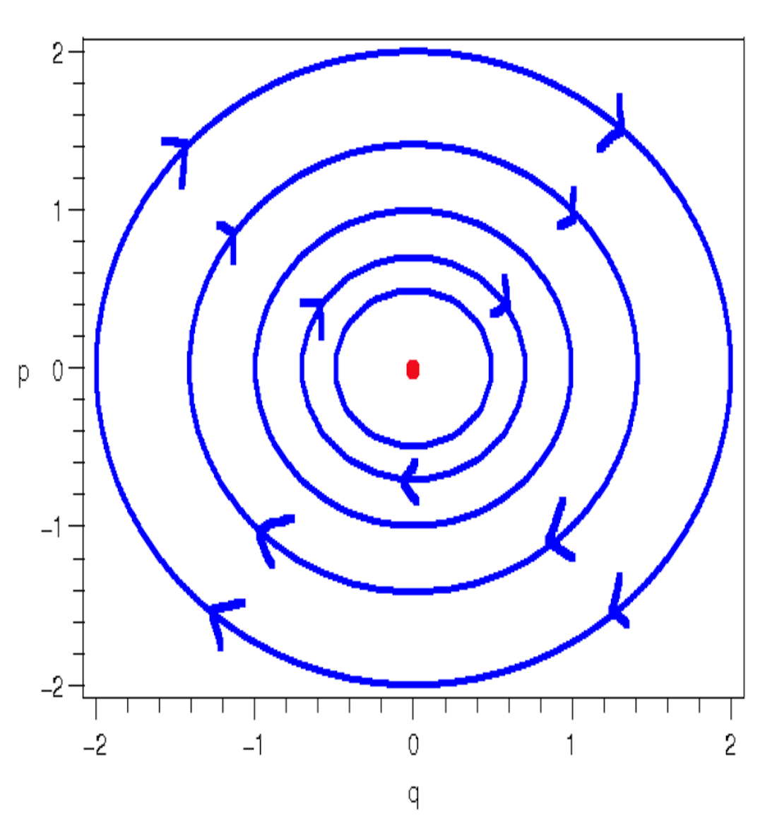
0.8.7 Poisson Brackets
Given a system of particles with generalized coordinates ,
and the Hamiltonian of the system,
the Poisson bracket of two functions %22%2F%3E%3C%2Fg%3E%3C%2Fg%3E%3Cdefs%3E%3Csymbol%20id%3D%22a%22%20overflow%3D%22visible%22%3E%3Cpath%20d%3D%22M8.28%209.495c0%20.66-.645%201.08-1.35%201.08-.93%200-1.575-.6-1.92-1.785-.075-.27-.24-1.035-.48-2.295h-.975c-.33%200-.495-.015-.495-.33%200-.165.15-.24.465-.24h.9L3.33.12c-.165-.855-.315-1.485-.45-1.905-.18-.555-.435-.84-.765-.84-.225%200-.405.06-.57.165.48.075.72.36.72.84%200%20.39-.195.585-.6.585-.51%200-.87-.45-.87-.96%200-.66.615-1.08%201.32-1.08.375%200%20.72.15%201.005.465.48.495.855%201.2%201.125%202.145.165.585.315%201.155.42%201.725l.87%204.665h1.23c.345%200%20.495.015.495.36%200%20.135-.15.21-.45.21H5.655c.09.615.51%202.88.645%203.165.15.315.36.465.63.465.225%200%20.42-.06.585-.165-.465-.105-.705-.375-.705-.84%200-.39.195-.585.6-.585.51%200%20.87.45.87.96%22%2F%3E%3C%2Fsymbol%3E%3C%2Fdefs%3E%3C%2Fsvg%3E) and of the phase space of the system is given by:
and of the phase space of the system is given by:

0.8.7.1 Properties of Poisson Brackets
Given a system of particles with generalized coordinates ,
and the Hamiltonian of the system,
the Poisson bracket of two functions and of the phase space of the system has the following properties:
- Antisymmetry:
%22%2F%3E%3Cuse%20xlink%3Ahref%3D%22%23b%22%20class%3D%22typst-text%22%20transform%3D%22matrix(1%200%200%20-1%208.5%2012.25)%22%2F%3E%3Cuse%20xlink%3Ahref%3D%22%23c%22%20class%3D%22typst-text%22%20transform%3D%22matrix(1%200%200%20-1%2017.2%2012.25)%22%2F%3E%3Cuse%20xlink%3Ahref%3D%22%23d%22%20class%3D%22typst-text%22%20transform%3D%22matrix(1%200%200%20-1%2023.87%2012.25)%22%2F%3E%3Cuse%20xlink%3Ahref%3D%22%23e%22%20class%3D%22typst-text%22%20transform%3D%22matrix(1%200%200%20-1%2031.4%2012.25)%22%2F%3E%3Cuse%20xlink%3Ahref%3D%22%23f%22%20class%3D%22typst-text%22%20transform%3D%22matrix(1%200%200%20-1%2043.067%2012.25)%22%2F%3E%3Cuse%20xlink%3Ahref%3D%22%23g%22%20class%3D%22typst-text%22%20transform%3D%22matrix(1%200%200%20-1%2058.903%2012.25)%22%2F%3E%3Cuse%20xlink%3Ahref%3D%22%23a%22%20class%3D%22typst-text%22%20transform%3D%22matrix(1%200%200%20-1%2070.573%2012.25)%22%2F%3E%3Cuse%20xlink%3Ahref%3D%22%23d%22%20class%3D%22typst-text%22%20transform%3D%22matrix(1%200%200%20-1%2078.073%2012.25)%22%2F%3E%3Cuse%20xlink%3Ahref%3D%22%23c%22%20class%3D%22typst-text%22%20transform%3D%22matrix(1%200%200%20-1%2085.603%2012.25)%22%2F%3E%3Cuse%20xlink%3Ahref%3D%22%23b%22%20class%3D%22typst-text%22%20transform%3D%22matrix(1%200%200%20-1%2092.273%2012.25)%22%2F%3E%3Cuse%20xlink%3Ahref%3D%22%23e%22%20class%3D%22typst-text%22%20transform%3D%22matrix(1%200%200%20-1%20100.973%2012.25)%22%2F%3E%3C%2Fg%3E%3C%2Fg%3E%3Cdefs%3E%3Csymbol%20id%3D%22a%22%20overflow%3D%22visible%22%3E%3Cpath%20d%3D%22M4.29-1.83v3.72c0%20.855-.525%201.485-1.56%201.86%201.035.375%201.56%201.005%201.56%201.86v3.72c0%20.87.93%201.44%201.845%201.44.165%200%20.24.075.24.24s-.075.24-.24.24c-.69%200-1.32-.15-1.875-.435-.705-.36-1.05-.855-1.05-1.485V5.61c0-.945-.9-1.62-1.845-1.62-.165%200-.24-.075-.24-.24s.075-.24.24-.24c.96%200%201.845-.69%201.845-1.62v-3.72c0-.63.345-1.125%201.05-1.485a4.06%204.06%200%200%201%201.875-.435c.165%200%20.24.075.24.24s-.075.24-.24.24c-.915%200-1.845.57-1.845%201.44%22%2F%3E%3C%2Fsymbol%3E%3Csymbol%20id%3D%22b%22%20overflow%3D%22visible%22%3E%3Cpath%20d%3D%22M8.28%209.495c0%20.66-.645%201.08-1.35%201.08-.93%200-1.575-.6-1.92-1.785-.075-.27-.24-1.035-.48-2.295h-.975c-.33%200-.495-.015-.495-.33%200-.165.15-.24.465-.24h.9L3.33.12c-.165-.855-.315-1.485-.45-1.905-.18-.555-.435-.84-.765-.84-.225%200-.405.06-.57.165.48.075.72.36.72.84%200%20.39-.195.585-.6.585-.51%200-.87-.45-.87-.96%200-.66.615-1.08%201.32-1.08.375%200%20.72.15%201.005.465.48.495.855%201.2%201.125%202.145.165.585.315%201.155.42%201.725l.87%204.665h1.23c.345%200%20.495.015.495.36%200%20.135-.15.21-.45.21H5.655c.09.615.51%202.88.645%203.165.15.315.36.465.63.465.225%200%20.42-.06.585-.165-.465-.105-.705-.375-.705-.84%200-.39.195-.585.6-.585.51%200%20.87.45.87.96%22%2F%3E%3C%2Fsymbol%3E%3Csymbol%20id%3D%22c%22%20overflow%3D%22visible%22%3E%3Cpath%20d%3D%22M2.085%201.59c-.48%200-.795-.36-.795-.84%200-.45.345-.825.795-.825.21%200%20.39.06.525.195L2.625%200c0-.945-.315-1.755-.945-2.4-.105-.12-.165-.21-.165-.27%200-.15.06-.225.195-.225s.315.18.57.525c.51.72.765%201.515.765%202.37%200%20.795-.27%201.59-.96%201.59%22%2F%3E%3C%2Fsymbol%3E%3Csymbol%20id%3D%22d%22%20overflow%3D%22visible%22%3E%3Cpath%20d%3D%22M.225-2.115c0-.645.675-.96%202.025-.96a3.8%203.8%200%200%201%201.95.525c.66.39%201.065.915%201.23%201.56l1.635%206.585c.03.15.045.24.045.285%200%20.3-.165.45-.48.45-.33%200-.54-.18-.645-.525-.33.555-.78.825-1.335.825-.96%200-1.815-.48-2.55-1.44-.675-.9-1.02-1.845-1.02-2.82%200-1.305.765-2.415%202.025-2.415.585%200%201.125.255%201.62.75l-.45-1.77C3.84-2.1%203.165-2.625%202.22-2.625q-.585%200-.99.09c.315.165.465.42.465.765%200%20.375-.21.57-.615.57-.48%200-.855-.435-.855-.915M5.34%205.88c.3-.315.45-.615.45-.915a1.3%201.3%200%200%200-.045-.195L5.04%201.935C4.95%201.59%204.695%201.23%204.29.9S3.495.405%203.15.405q-.9%200-.9%201.305c0%20.825.51%202.655.81%203.195.465.855.99%201.275%201.605%201.275.27%200%20.495-.105.675-.3%22%2F%3E%3C%2Fsymbol%3E%3Csymbol%20id%3D%22e%22%20overflow%3D%22visible%22%3E%3Cpath%20d%3D%22M4.29%205.61v3.72c0%20.63-.345%201.125-1.05%201.485a4.06%204.06%200%200%201-1.875.435c-.165%200-.24-.075-.24-.24s.075-.24.24-.24c.915%200%201.845-.57%201.845-1.44V5.61c0-.855.525-1.485%201.56-1.86-1.035-.375-1.56-1.005-1.56-1.86v-3.72c0-.87-.93-1.44-1.845-1.44-.165%200-.24-.075-.24-.24s.075-.24.24-.24c.69%200%201.32.15%201.875.435.705.36%201.05.855%201.05%201.485v3.72c0%20.93.885%201.62%201.845%201.62.165%200%20.24.075.24.24s-.075.24-.24.24c-.96%200-1.845.69-1.845%201.62%22%2F%3E%3C%2Fsymbol%3E%3Csymbol%20id%3D%22f%22%20overflow%3D%22visible%22%3E%3Cpath%20d%3D%22M10.47%205.505H1.2c-.24%200-.36-.12-.36-.345s.12-.345.36-.345h9.27c.24%200%20.36.12.36.345%200%20.18-.165.345-.36.345m0-2.82H1.2c-.24%200-.36-.12-.36-.345s.12-.345.36-.345h9.27c.24%200%20.36.12.36.345a.35.35%200%200%201-.36.345%22%2F%3E%3C%2Fsymbol%3E%3Csymbol%20id%3D%22g%22%20overflow%3D%22visible%22%3E%3Cpath%20d%3D%22M10.47%204.05H1.2c-.24%200-.36-.105-.36-.3s.12-.3.36-.3h9.27c.24%200%20.36.105.36.3%200%20.18-.18.3-.36.3%22%2F%3E%3C%2Fsymbol%3E%3C%2Fdefs%3E%3C%2Fsvg%3E)
- Linearity:
%22%2F%3E%3Cuse%20xlink%3Ahref%3D%22%23b%22%20class%3D%22typst-text%22%20transform%3D%22matrix(1%200%200%20-1%208.5%2012.25)%22%2F%3E%3Cuse%20xlink%3Ahref%3D%22%23c%22%20class%3D%22typst-text%22%20transform%3D%22matrix(1%200%200%20-1%2016.435%2012.25)%22%2F%3E%3Cuse%20xlink%3Ahref%3D%22%23d%22%20class%3D%22typst-text%22%20transform%3D%22matrix(1%200%200%20-1%2028.468%2012.25)%22%2F%3E%3Cuse%20xlink%3Ahref%3D%22%23e%22%20class%3D%22typst-text%22%20transform%3D%22matrix(1%200%200%20-1%2043.472%2012.25)%22%2F%3E%3Cuse%20xlink%3Ahref%3D%22%23f%22%20class%3D%22typst-text%22%20transform%3D%22matrix(1%200%200%20-1%2050.117%2012.25)%22%2F%3E%3Cuse%20xlink%3Ahref%3D%22%23g%22%20class%3D%22typst-text%22%20transform%3D%22matrix(1%200%200%20-1%2057.647%2012.25)%22%2F%3E%3Cuse%20xlink%3Ahref%3D%22%23h%22%20class%3D%22typst-text%22%20transform%3D%22matrix(1%200%200%20-1%2064.317%2012.25)%22%2F%3E%3Cuse%20xlink%3Ahref%3D%22%23i%22%20class%3D%22typst-text%22%20transform%3D%22matrix(1%200%200%20-1%2072.957%2012.25)%22%2F%3E%3Cuse%20xlink%3Ahref%3D%22%23j%22%20class%3D%22typst-text%22%20transform%3D%22matrix(1%200%200%20-1%2084.623%2012.25)%22%2F%3E%3Cuse%20xlink%3Ahref%3D%22%23b%22%20class%3D%22typst-text%22%20transform%3D%22matrix(1%200%200%20-1%20100.46%2012.25)%22%2F%3E%3Cuse%20xlink%3Ahref%3D%22%23a%22%20class%3D%22typst-text%22%20transform%3D%22matrix(1%200%200%20-1%20108.395%2012.25)%22%2F%3E%3Cuse%20xlink%3Ahref%3D%22%23c%22%20class%3D%22typst-text%22%20transform%3D%22matrix(1%200%200%20-1%20115.895%2012.25)%22%2F%3E%3Cuse%20xlink%3Ahref%3D%22%23g%22%20class%3D%22typst-text%22%20transform%3D%22matrix(1%200%200%20-1%20124.595%2012.25)%22%2F%3E%3Cuse%20xlink%3Ahref%3D%22%23h%22%20class%3D%22typst-text%22%20transform%3D%22matrix(1%200%200%20-1%20131.265%2012.25)%22%2F%3E%3Cuse%20xlink%3Ahref%3D%22%23i%22%20class%3D%22typst-text%22%20transform%3D%22matrix(1%200%200%20-1%20139.905%2012.25)%22%2F%3E%3Cuse%20xlink%3Ahref%3D%22%23d%22%20class%3D%22typst-text%22%20transform%3D%22matrix(1%200%200%20-1%20150.738%2012.25)%22%2F%3E%3Cuse%20xlink%3Ahref%3D%22%23e%22%20class%3D%22typst-text%22%20transform%3D%22matrix(1%200%200%20-1%20165.742%2012.25)%22%2F%3E%3Cuse%20xlink%3Ahref%3D%22%23a%22%20class%3D%22typst-text%22%20transform%3D%22matrix(1%200%200%20-1%20172.387%2012.25)%22%2F%3E%3Cuse%20xlink%3Ahref%3D%22%23f%22%20class%3D%22typst-text%22%20transform%3D%22matrix(1%200%200%20-1%20179.887%2012.25)%22%2F%3E%3Cuse%20xlink%3Ahref%3D%22%23g%22%20class%3D%22typst-text%22%20transform%3D%22matrix(1%200%200%20-1%20187.417%2012.25)%22%2F%3E%3Cuse%20xlink%3Ahref%3D%22%23h%22%20class%3D%22typst-text%22%20transform%3D%22matrix(1%200%200%20-1%20194.087%2012.25)%22%2F%3E%3Cuse%20xlink%3Ahref%3D%22%23i%22%20class%3D%22typst-text%22%20transform%3D%22matrix(1%200%200%20-1%20202.727%2012.25)%22%2F%3E%3C%2Fg%3E%3C%2Fg%3E%3Cdefs%3E%3Csymbol%20id%3D%22a%22%20overflow%3D%22visible%22%3E%3Cpath%20d%3D%22M4.29-1.83v3.72c0%20.855-.525%201.485-1.56%201.86%201.035.375%201.56%201.005%201.56%201.86v3.72c0%20.87.93%201.44%201.845%201.44.165%200%20.24.075.24.24s-.075.24-.24.24c-.69%200-1.32-.15-1.875-.435-.705-.36-1.05-.855-1.05-1.485V5.61c0-.945-.9-1.62-1.845-1.62-.165%200-.24-.075-.24-.24s.075-.24.24-.24c.96%200%201.845-.69%201.845-1.62v-3.72c0-.63.345-1.125%201.05-1.485a4.06%204.06%200%200%201%201.875-.435c.165%200%20.24.075.24.24s-.075.24-.24.24c-.915%200-1.845.57-1.845%201.44%22%2F%3E%3C%2Fsymbol%3E%3Csymbol%20id%3D%22b%22%20overflow%3D%22visible%22%3E%3Cpath%20d%3D%22M7.47%202.16c0%20.135-.075.21-.24.21-.12%200-.21-.105-.255-.315C6.675.87%206.315.27%205.91.27c-.255%200-.39.21-.39.63%200%20.195.06.555.195%201.08l.855%203.375c.075.285.105.45.105.525q0%20.45-.495.45c-.315%200-.525-.18-.63-.525-.315.555-.765.825-1.335.825-.975%200-1.83-.495-2.58-1.485C.945%204.215.6%203.255.6%202.25.6.945%201.365-.165%202.625-.165%203.27-.165%203.9.18%204.5.87A1.416%201.416%200%200%201%205.88-.165c1.035%200%201.35%201.215%201.59%202.325M5.115%205.61c.135-.315.21-.525.21-.66%200-.06-.015-.135-.03-.24L4.56%201.83a1.7%201.7%200%200%200-.285-.525Q3.443.27%202.655.27c-.585%200-.885.45-.885%201.335q0%20.54.27%201.62c.315%201.275.765%202.13%201.32%202.595.3.255.585.375.87.375.405%200%20.705-.195.885-.585%22%2F%3E%3C%2Fsymbol%3E%3Csymbol%20id%3D%22c%22%20overflow%3D%22visible%22%3E%3Cpath%20d%3D%22M8.28%209.495c0%20.66-.645%201.08-1.35%201.08-.93%200-1.575-.6-1.92-1.785-.075-.27-.24-1.035-.48-2.295h-.975c-.33%200-.495-.015-.495-.33%200-.165.15-.24.465-.24h.9L3.33.12c-.165-.855-.315-1.485-.45-1.905-.18-.555-.435-.84-.765-.84-.225%200-.405.06-.57.165.48.075.72.36.72.84%200%20.39-.195.585-.6.585-.51%200-.87-.45-.87-.96%200-.66.615-1.08%201.32-1.08.375%200%20.72.15%201.005.465.48.495.855%201.2%201.125%202.145.165.585.315%201.155.42%201.725l.87%204.665h1.23c.345%200%20.495.015.495.36%200%20.135-.15.21-.45.21H5.655c.09.615.51%202.88.645%203.165.15.315.36.465.63.465.225%200%20.42-.06.585-.165-.465-.105-.705-.375-.705-.84%200-.39.195-.585.6-.585.51%200%20.87.45.87.96%22%2F%3E%3C%2Fsymbol%3E%3Csymbol%20id%3D%22d%22%20overflow%3D%22visible%22%3E%3Cpath%20d%3D%22M10.47%204.11H6.195v4.275q0%20.36-.36.36t-.36-.36V4.11H1.2q-.36%200-.36-.36t.36-.36h4.275V-.885q0-.36.36-.36t.36.36V3.39h4.275q.36%200%20.36.36c0%20.195-.165.36-.36.36%22%2F%3E%3C%2Fsymbol%3E%3Csymbol%20id%3D%22e%22%20overflow%3D%22visible%22%3E%3Cpath%20d%3D%22M4.215%206.675c-.54%200-1.08-.255-1.605-.765l1.035%204.275c-.03.135-.075.225-.255.225-.495%200-1.59-.135-1.785-.15-.225-.03-.345-.135-.345-.36%200-.15.135-.225.42-.225s.675.015.675-.195c0-.06-.075-.36-.21-.915l-1.2-4.83c-.165-.63-.24-1.14-.24-1.515%200-1.29.69-2.385%201.92-2.385.975%200%201.83.495%202.58%201.5.675.93%201.02%201.905%201.02%202.91%200%201.305-.765%202.43-2.01%202.43m-.03-.45c.585%200%20.87-.45.87-1.335q0-.608-.27-1.62c-.33-1.275-.765-2.145-1.29-2.61-.3-.255-.585-.375-.87-.375-.615%200-.915.48-.915%201.44q0%20.495.225%201.485l.33%201.35c.045.225.12.39.21.51.585.765%201.155%201.155%201.71%201.155%22%2F%3E%3C%2Fsymbol%3E%3Csymbol%20id%3D%22f%22%20overflow%3D%22visible%22%3E%3Cpath%20d%3D%22M.225-2.115c0-.645.675-.96%202.025-.96a3.8%203.8%200%200%201%201.95.525c.66.39%201.065.915%201.23%201.56l1.635%206.585c.03.15.045.24.045.285%200%20.3-.165.45-.48.45-.33%200-.54-.18-.645-.525-.33.555-.78.825-1.335.825-.96%200-1.815-.48-2.55-1.44-.675-.9-1.02-1.845-1.02-2.82%200-1.305.765-2.415%202.025-2.415.585%200%201.125.255%201.62.75l-.45-1.77C3.84-2.1%203.165-2.625%202.22-2.625q-.585%200-.99.09c.315.165.465.42.465.765%200%20.375-.21.57-.615.57-.48%200-.855-.435-.855-.915M5.34%205.88c.3-.315.45-.615.45-.915a1.3%201.3%200%200%200-.045-.195L5.04%201.935C4.95%201.59%204.695%201.23%204.29.9S3.495.405%203.15.405q-.9%200-.9%201.305c0%20.825.51%202.655.81%203.195.465.855.99%201.275%201.605%201.275.27%200%20.495-.105.675-.3%22%2F%3E%3C%2Fsymbol%3E%3Csymbol%20id%3D%22g%22%20overflow%3D%22visible%22%3E%3Cpath%20d%3D%22M2.085%201.59c-.48%200-.795-.36-.795-.84%200-.45.345-.825.795-.825.21%200%20.39.06.525.195L2.625%200c0-.945-.315-1.755-.945-2.4-.105-.12-.165-.21-.165-.27%200-.15.06-.225.195-.225s.315.18.57.525c.51.72.765%201.515.765%202.37%200%20.795-.27%201.59-.96%201.59%22%2F%3E%3C%2Fsymbol%3E%3Csymbol%20id%3D%22h%22%20overflow%3D%22visible%22%3E%3Cpath%20d%3D%22M7.68%202.07C7.335.885%206.855.285%206.225.285c-.195%200-.3.135-.3.42q0%20.338.27%201.035.9%202.407.9%203.285c0%201.065-.69%201.65-1.755%201.65-.795%200-1.485-.33-2.07-.975l1.095%204.485c-.03.135-.06.225-.255.225-.495%200-1.59-.135-1.785-.15-.225-.03-.345-.135-.345-.36q0-.225.405-.225c.315%200%20.66.015.69-.195L.885.645a1.4%201.4%200%200%201-.06-.33c0-.315.165-.48.48-.48.3%200%20.51.15.615.435l.6%202.46c.18.735.315%201.29.42%201.665.045.105.165.315.36.615.54.81%201.2%201.215%201.995%201.215.495%200%20.735-.33.735-.975%200-.615-.3-1.71-.9-3.3-.135-.345-.195-.615-.195-.84%200-.72.54-1.275%201.26-1.275.66%200%201.185.375%201.56%201.14.285.6.435%201.005.435%201.2%200%20.135-.075.21-.24.21-.045%200-.27-.135-.27-.315%22%2F%3E%3C%2Fsymbol%3E%3Csymbol%20id%3D%22i%22%20overflow%3D%22visible%22%3E%3Cpath%20d%3D%22M4.29%205.61v3.72c0%20.63-.345%201.125-1.05%201.485a4.06%204.06%200%200%201-1.875.435c-.165%200-.24-.075-.24-.24s.075-.24.24-.24c.915%200%201.845-.57%201.845-1.44V5.61c0-.855.525-1.485%201.56-1.86-1.035-.375-1.56-1.005-1.56-1.86v-3.72c0-.87-.93-1.44-1.845-1.44-.165%200-.24-.075-.24-.24s.075-.24.24-.24c.69%200%201.32.15%201.875.435.705.36%201.05.855%201.05%201.485v3.72c0%20.93.885%201.62%201.845%201.62.165%200%20.24.075.24.24s-.075.24-.24.24c-.96%200-1.845.69-1.845%201.62%22%2F%3E%3C%2Fsymbol%3E%3Csymbol%20id%3D%22j%22%20overflow%3D%22visible%22%3E%3Cpath%20d%3D%22M10.47%205.505H1.2c-.24%200-.36-.12-.36-.345s.12-.345.36-.345h9.27c.24%200%20.36.12.36.345%200%20.18-.165.345-.36.345m0-2.82H1.2c-.24%200-.36-.12-.36-.345s.12-.345.36-.345h9.27c.24%200%20.36.12.36.345a.35.35%200%200%201-.36.345%22%2F%3E%3C%2Fsymbol%3E%3C%2Fdefs%3E%3C%2Fsvg%3E)
- Product(Leibnitz) Rule:
%22%2F%3E%3Cuse%20xlink%3Ahref%3D%22%23b%22%20class%3D%22typst-text%22%20transform%3D%22matrix(1%200%200%20-1%208.5%2012.25)%22%2F%3E%3Cuse%20xlink%3Ahref%3D%22%23c%22%20class%3D%22typst-text%22%20transform%3D%22matrix(1%200%200%20-1%2017.2%2012.25)%22%2F%3E%3Cuse%20xlink%3Ahref%3D%22%23d%22%20class%3D%22typst-text%22%20transform%3D%22matrix(1%200%200%20-1%2024.73%2012.25)%22%2F%3E%3Cuse%20xlink%3Ahref%3D%22%23e%22%20class%3D%22typst-text%22%20transform%3D%22matrix(1%200%200%20-1%2031.4%2012.25)%22%2F%3E%3Cuse%20xlink%3Ahref%3D%22%23f%22%20class%3D%22typst-text%22%20transform%3D%22matrix(1%200%200%20-1%2040.04%2012.25)%22%2F%3E%3Cuse%20xlink%3Ahref%3D%22%23g%22%20class%3D%22typst-text%22%20transform%3D%22matrix(1%200%200%20-1%2051.707%2012.25)%22%2F%3E%3Cuse%20xlink%3Ahref%3D%22%23b%22%20class%3D%22typst-text%22%20transform%3D%22matrix(1%200%200%20-1%2067.543%2012.25)%22%2F%3E%3Cuse%20xlink%3Ahref%3D%22%23a%22%20class%3D%22typst-text%22%20transform%3D%22matrix(1%200%200%20-1%2076.243%2012.25)%22%2F%3E%3Cuse%20xlink%3Ahref%3D%22%23c%22%20class%3D%22typst-text%22%20transform%3D%22matrix(1%200%200%20-1%2083.743%2012.25)%22%2F%3E%3Cuse%20xlink%3Ahref%3D%22%23d%22%20class%3D%22typst-text%22%20transform%3D%22matrix(1%200%200%20-1%2091.273%2012.25)%22%2F%3E%3Cuse%20xlink%3Ahref%3D%22%23e%22%20class%3D%22typst-text%22%20transform%3D%22matrix(1%200%200%20-1%2097.943%2012.25)%22%2F%3E%3Cuse%20xlink%3Ahref%3D%22%23f%22%20class%3D%22typst-text%22%20transform%3D%22matrix(1%200%200%20-1%20106.583%2012.25)%22%2F%3E%3Cuse%20xlink%3Ahref%3D%22%23h%22%20class%3D%22typst-text%22%20transform%3D%22matrix(1%200%200%20-1%20117.417%2012.25)%22%2F%3E%3Cuse%20xlink%3Ahref%3D%22%23c%22%20class%3D%22typst-text%22%20transform%3D%22matrix(1%200%200%20-1%20132.42%2012.25)%22%2F%3E%3Cuse%20xlink%3Ahref%3D%22%23a%22%20class%3D%22typst-text%22%20transform%3D%22matrix(1%200%200%20-1%20139.95%2012.25)%22%2F%3E%3Cuse%20xlink%3Ahref%3D%22%23b%22%20class%3D%22typst-text%22%20transform%3D%22matrix(1%200%200%20-1%20147.45%2012.25)%22%2F%3E%3Cuse%20xlink%3Ahref%3D%22%23d%22%20class%3D%22typst-text%22%20transform%3D%22matrix(1%200%200%20-1%20156.15%2012.25)%22%2F%3E%3Cuse%20xlink%3Ahref%3D%22%23e%22%20class%3D%22typst-text%22%20transform%3D%22matrix(1%200%200%20-1%20162.82%2012.25)%22%2F%3E%3Cuse%20xlink%3Ahref%3D%22%23f%22%20class%3D%22typst-text%22%20transform%3D%22matrix(1%200%200%20-1%20171.46%2012.25)%22%2F%3E%3C%2Fg%3E%3C%2Fg%3E%3Cdefs%3E%3Csymbol%20id%3D%22a%22%20overflow%3D%22visible%22%3E%3Cpath%20d%3D%22M4.29-1.83v3.72c0%20.855-.525%201.485-1.56%201.86%201.035.375%201.56%201.005%201.56%201.86v3.72c0%20.87.93%201.44%201.845%201.44.165%200%20.24.075.24.24s-.075.24-.24.24c-.69%200-1.32-.15-1.875-.435-.705-.36-1.05-.855-1.05-1.485V5.61c0-.945-.9-1.62-1.845-1.62-.165%200-.24-.075-.24-.24s.075-.24.24-.24c.96%200%201.845-.69%201.845-1.62v-3.72c0-.63.345-1.125%201.05-1.485a4.06%204.06%200%200%201%201.875-.435c.165%200%20.24.075.24.24s-.075.24-.24.24c-.915%200-1.845.57-1.845%201.44%22%2F%3E%3C%2Fsymbol%3E%3Csymbol%20id%3D%22b%22%20overflow%3D%22visible%22%3E%3Cpath%20d%3D%22M8.28%209.495c0%20.66-.645%201.08-1.35%201.08-.93%200-1.575-.6-1.92-1.785-.075-.27-.24-1.035-.48-2.295h-.975c-.33%200-.495-.015-.495-.33%200-.165.15-.24.465-.24h.9L3.33.12c-.165-.855-.315-1.485-.45-1.905-.18-.555-.435-.84-.765-.84-.225%200-.405.06-.57.165.48.075.72.36.72.84%200%20.39-.195.585-.6.585-.51%200-.87-.45-.87-.96%200-.66.615-1.08%201.32-1.08.375%200%20.72.15%201.005.465.48.495.855%201.2%201.125%202.145.165.585.315%201.155.42%201.725l.87%204.665h1.23c.345%200%20.495.015.495.36%200%20.135-.15.21-.45.21H5.655c.09.615.51%202.88.645%203.165.15.315.36.465.63.465.225%200%20.42-.06.585-.165-.465-.105-.705-.375-.705-.84%200-.39.195-.585.6-.585.51%200%20.87.45.87.96%22%2F%3E%3C%2Fsymbol%3E%3Csymbol%20id%3D%22c%22%20overflow%3D%22visible%22%3E%3Cpath%20d%3D%22M.225-2.115c0-.645.675-.96%202.025-.96a3.8%203.8%200%200%201%201.95.525c.66.39%201.065.915%201.23%201.56l1.635%206.585c.03.15.045.24.045.285%200%20.3-.165.45-.48.45-.33%200-.54-.18-.645-.525-.33.555-.78.825-1.335.825-.96%200-1.815-.48-2.55-1.44-.675-.9-1.02-1.845-1.02-2.82%200-1.305.765-2.415%202.025-2.415.585%200%201.125.255%201.62.75l-.45-1.77C3.84-2.1%203.165-2.625%202.22-2.625q-.585%200-.99.09c.315.165.465.42.465.765%200%20.375-.21.57-.615.57-.48%200-.855-.435-.855-.915M5.34%205.88c.3-.315.45-.615.45-.915a1.3%201.3%200%200%200-.045-.195L5.04%201.935C4.95%201.59%204.695%201.23%204.29.9S3.495.405%203.15.405q-.9%200-.9%201.305c0%20.825.51%202.655.81%203.195.465.855.99%201.275%201.605%201.275.27%200%20.495-.105.675-.3%22%2F%3E%3C%2Fsymbol%3E%3Csymbol%20id%3D%22d%22%20overflow%3D%22visible%22%3E%3Cpath%20d%3D%22M2.085%201.59c-.48%200-.795-.36-.795-.84%200-.45.345-.825.795-.825.21%200%20.39.06.525.195L2.625%200c0-.945-.315-1.755-.945-2.4-.105-.12-.165-.21-.165-.27%200-.15.06-.225.195-.225s.315.18.57.525c.51.72.765%201.515.765%202.37%200%20.795-.27%201.59-.96%201.59%22%2F%3E%3C%2Fsymbol%3E%3Csymbol%20id%3D%22e%22%20overflow%3D%22visible%22%3E%3Cpath%20d%3D%22M7.68%202.07C7.335.885%206.855.285%206.225.285c-.195%200-.3.135-.3.42q0%20.338.27%201.035.9%202.407.9%203.285c0%201.065-.69%201.65-1.755%201.65-.795%200-1.485-.33-2.07-.975l1.095%204.485c-.03.135-.06.225-.255.225-.495%200-1.59-.135-1.785-.15-.225-.03-.345-.135-.345-.36q0-.225.405-.225c.315%200%20.66.015.69-.195L.885.645a1.4%201.4%200%200%201-.06-.33c0-.315.165-.48.48-.48.3%200%20.51.15.615.435l.6%202.46c.18.735.315%201.29.42%201.665.045.105.165.315.36.615.54.81%201.2%201.215%201.995%201.215.495%200%20.735-.33.735-.975%200-.615-.3-1.71-.9-3.3-.135-.345-.195-.615-.195-.84%200-.72.54-1.275%201.26-1.275.66%200%201.185.375%201.56%201.14.285.6.435%201.005.435%201.2%200%20.135-.075.21-.24.21-.045%200-.27-.135-.27-.315%22%2F%3E%3C%2Fsymbol%3E%3Csymbol%20id%3D%22f%22%20overflow%3D%22visible%22%3E%3Cpath%20d%3D%22M4.29%205.61v3.72c0%20.63-.345%201.125-1.05%201.485a4.06%204.06%200%200%201-1.875.435c-.165%200-.24-.075-.24-.24s.075-.24.24-.24c.915%200%201.845-.57%201.845-1.44V5.61c0-.855.525-1.485%201.56-1.86-1.035-.375-1.56-1.005-1.56-1.86v-3.72c0-.87-.93-1.44-1.845-1.44-.165%200-.24-.075-.24-.24s.075-.24.24-.24c.69%200%201.32.15%201.875.435.705.36%201.05.855%201.05%201.485v3.72c0%20.93.885%201.62%201.845%201.62.165%200%20.24.075.24.24s-.075.24-.24.24c-.96%200-1.845.69-1.845%201.62%22%2F%3E%3C%2Fsymbol%3E%3Csymbol%20id%3D%22g%22%20overflow%3D%22visible%22%3E%3Cpath%20d%3D%22M10.47%205.505H1.2c-.24%200-.36-.12-.36-.345s.12-.345.36-.345h9.27c.24%200%20.36.12.36.345%200%20.18-.165.345-.36.345m0-2.82H1.2c-.24%200-.36-.12-.36-.345s.12-.345.36-.345h9.27c.24%200%20.36.12.36.345a.35.35%200%200%201-.36.345%22%2F%3E%3C%2Fsymbol%3E%3Csymbol%20id%3D%22h%22%20overflow%3D%22visible%22%3E%3Cpath%20d%3D%22M10.47%204.11H6.195v4.275q0%20.36-.36.36t-.36-.36V4.11H1.2q-.36%200-.36-.36t.36-.36h4.275V-.885q0-.36.36-.36t.36.36V3.39h4.275q.36%200%20.36.36c0%20.195-.165.36-.36.36%22%2F%3E%3C%2Fsymbol%3E%3C%2Fdefs%3E%3C%2Fsvg%3E)
0.8.7.2 Fundamental Poisson Brackets
Given a system of particles with generalized coordinates ,
and the Hamiltonian of the system,
the fundamental Poisson brackets of the system are given by:

0.8.7.3 Constant of Motion and Poisson Brackets
Given a system of particles with generalized coordinates ,
and the Hamiltonian of the system,
and a function of the phase space of the system,
then time derivative of the function is given by:
%22%2F%3E%3Cuse%20xlink%3Ahref%3D%22%23b%22%20class%3D%22typst-text%22%20transform%3D%22matrix(1%200%200%20-1%2019.66%2016.915)%22%2F%3E%3Cuse%20xlink%3Ahref%3D%22%23a%22%20class%3D%22typst-text%22%20transform%3D%22matrix(1%200%200%20-1%2013.143%2037.36)%22%2F%3E%3Cuse%20xlink%3Ahref%3D%22%23c%22%20class%3D%22typst-text%22%20transform%3D%22matrix(1%200%200%20-1%2021.303%2037.36)%22%2F%3E%3Cpath%20fill%3D%22none%22%20stroke%3D%22%23000%22%20stroke-width%3D%22.72%22%20d%3D%22M11.5%2023.32h16.86%22%20class%3D%22typst-shape%22%2F%3E%3Cuse%20xlink%3Ahref%3D%22%23d%22%20class%3D%22typst-text%22%20transform%3D%22matrix(1%200%200%20-1%2034.027%2027.07)%22%2F%3E%3Cuse%20xlink%3Ahref%3D%22%23e%22%20class%3D%22typst-text%22%20transform%3D%22matrix(1%200%200%20-1%2049.863%2027.07)%22%2F%3E%3Cuse%20xlink%3Ahref%3D%22%23b%22%20class%3D%22typst-text%22%20transform%3D%22matrix(1%200%200%20-1%2057.363%2027.07)%22%2F%3E%3Cuse%20xlink%3Ahref%3D%22%23f%22%20class%3D%22typst-text%22%20transform%3D%22matrix(1%200%200%20-1%2066.063%2027.07)%22%2F%3E%3Cuse%20xlink%3Ahref%3D%22%23g%22%20class%3D%22typst-text%22%20transform%3D%22matrix(1%200%200%20-1%2072.733%2027.07)%22%2F%3E%3Cuse%20xlink%3Ahref%3D%22%23h%22%20class%3D%22typst-text%22%20transform%3D%22matrix(1%200%200%20-1%2086.368%2027.07)%22%2F%3E%3Cuse%20xlink%3Ahref%3D%22%23i%22%20class%3D%22typst-text%22%20transform%3D%22matrix(1%200%200%20-1%2097.202%2027.07)%22%2F%3E%3Cuse%20xlink%3Ahref%3D%22%23j%22%20class%3D%22typst-text%22%20transform%3D%22matrix(1%200%200%20-1%20113.705%2016.915)%22%2F%3E%3Cuse%20xlink%3Ahref%3D%22%23b%22%20class%3D%22typst-text%22%20transform%3D%22matrix(1%200%200%20-1%20122.615%2016.915)%22%2F%3E%3Cuse%20xlink%3Ahref%3D%22%23j%22%20class%3D%22typst-text%22%20transform%3D%22matrix(1%200%200%20-1%20115.348%2037.36)%22%2F%3E%3Cuse%20xlink%3Ahref%3D%22%23c%22%20class%3D%22typst-text%22%20transform%3D%22matrix(1%200%200%20-1%20124.258%2037.36)%22%2F%3E%3Cpath%20fill%3D%22none%22%20stroke%3D%22%23000%22%20stroke-width%3D%22.72%22%20d%3D%22M113.705%2023.32h17.61%22%20class%3D%22typst-shape%22%2F%3E%3C%2Fg%3E%3C%2Fg%3E%3C%2Fg%3E%3C%2Fg%3E%3C%2Fg%3E%3Cdefs%3E%3Csymbol%20id%3D%22a%22%20overflow%3D%22visible%22%3E%3Cpath%20d%3D%22M6.435%209.48%205.55%205.835c-.315.555-.75.84-1.335.84-.975%200-1.83-.495-2.58-1.5C.945%204.245.6%203.27.6%202.265c0-1.32.765-2.43%202.025-2.43C3.27-.165%203.9.18%204.5.885c.165-.57.675-1.05%201.38-1.05%201.035%200%201.365%201.23%201.59%202.34%200%20.135-.075.21-.225.21q-.202%200-.27-.315C6.675.885%206.315.285%205.91.285c-.255%200-.39.21-.39.615%200%20.225.03.465.09.705l2.13%208.58v.06a.26.26%200%200%201-.255.165c-.345%200-.975-.06-1.875-.165-.165-.015-.255-.135-.255-.345q0-.225.405-.225c.285%200%20.675.015.675-.195m-1.32-3.84c.15-.315.225-.525.225-.66a2%202%200%200%201-.045-.24L4.56%201.83a1.7%201.7%200%200%200-.285-.525C3.72.63%203.18.285%202.655.285c-.585%200-.885.45-.885%201.335q0%20.54.27%201.62c.315%201.275.765%202.145%201.32%202.61.3.255.585.375.87.375.405%200%20.705-.195.885-.585%22%2F%3E%3C%2Fsymbol%3E%3Csymbol%20id%3D%22b%22%20overflow%3D%22visible%22%3E%3Cpath%20d%3D%22M8.28%209.495c0%20.66-.645%201.08-1.35%201.08-.93%200-1.575-.6-1.92-1.785-.075-.27-.24-1.035-.48-2.295h-.975c-.33%200-.495-.015-.495-.33%200-.165.15-.24.465-.24h.9L3.33.12c-.165-.855-.315-1.485-.45-1.905-.18-.555-.435-.84-.765-.84-.225%200-.405.06-.57.165.48.075.72.36.72.84%200%20.39-.195.585-.6.585-.51%200-.87-.45-.87-.96%200-.66.615-1.08%201.32-1.08.375%200%20.72.15%201.005.465.48.495.855%201.2%201.125%202.145.165.585.315%201.155.42%201.725l.87%204.665h1.23c.345%200%20.495.015.495.36%200%20.135-.15.21-.45.21H5.655c.09.615.51%202.88.645%203.165.15.315.36.465.63.465.225%200%20.42-.06.585-.165-.465-.105-.705-.375-.705-.84%200-.39.195-.585.6-.585.51%200%20.87.45.87.96%22%2F%3E%3C%2Fsymbol%3E%3Csymbol%20id%3D%22c%22%20overflow%3D%22visible%22%3E%3Cpath%20d%3D%22M4.95%206.285c0%20.135-.15.21-.465.21H3.27q.585%202.34.585%202.43c0%20.315-.165.465-.48.465-.345%200-.555-.195-.645-.585l-.555-2.31H.84c-.33%200-.495-.015-.495-.33%200-.165.15-.24.465-.24h1.215C1.29%203%20.93%201.455.93%201.26c0-.84.57-1.425%201.41-1.425.57%200%201.065.255%201.5.78.36.435.615.855.78%201.26.06.165.09.255.09.3%200%20.135-.075.21-.225.21-.12%200-.21-.075-.27-.24C3.705.9%203.09.285%202.355.285c-.255%200-.39.21-.39.615%200%20.225.03.465.09.705l1.065%204.32h1.335c.39%200%20.495.03.495.36%22%2F%3E%3C%2Fsymbol%3E%3Csymbol%20id%3D%22d%22%20overflow%3D%22visible%22%3E%3Cpath%20d%3D%22M10.47%205.505H1.2c-.24%200-.36-.12-.36-.345s.12-.345.36-.345h9.27c.24%200%20.36.12.36.345%200%20.18-.165.345-.36.345m0-2.82H1.2c-.24%200-.36-.12-.36-.345s.12-.345.36-.345h9.27c.24%200%20.36.12.36.345a.35.35%200%200%201-.36.345%22%2F%3E%3C%2Fsymbol%3E%3Csymbol%20id%3D%22e%22%20overflow%3D%22visible%22%3E%3Cpath%20d%3D%22M4.29-1.83v3.72c0%20.855-.525%201.485-1.56%201.86%201.035.375%201.56%201.005%201.56%201.86v3.72c0%20.87.93%201.44%201.845%201.44.165%200%20.24.075.24.24s-.075.24-.24.24c-.69%200-1.32-.15-1.875-.435-.705-.36-1.05-.855-1.05-1.485V5.61c0-.945-.9-1.62-1.845-1.62-.165%200-.24-.075-.24-.24s.075-.24.24-.24c.96%200%201.845-.69%201.845-1.62v-3.72c0-.63.345-1.125%201.05-1.485a4.06%204.06%200%200%201%201.875-.435c.165%200%20.24.075.24.24s-.075.24-.24.24c-.915%200-1.845.57-1.845%201.44%22%2F%3E%3C%2Fsymbol%3E%3Csymbol%20id%3D%22f%22%20overflow%3D%22visible%22%3E%3Cpath%20d%3D%22M2.085%201.59c-.48%200-.795-.36-.795-.84%200-.45.345-.825.795-.825.21%200%20.39.06.525.195L2.625%200c0-.945-.315-1.755-.945-2.4-.105-.12-.165-.21-.165-.27%200-.15.06-.225.195-.225s.315.18.57.525c.51.72.765%201.515.765%202.37%200%20.795-.27%201.59-.96%201.59%22%2F%3E%3C%2Fsymbol%3E%3Csymbol%20id%3D%22g%22%20overflow%3D%22visible%22%3E%3Cpath%20d%3D%22M13.215%2010.02q0%20.225-.27.225L11.04%2010.2l-1.905.045c-.24%200-.345-.135-.345-.36%200-.105.045-.18.12-.195.15-.015.27-.03.345-.03a6%206%200%200%200%20.795-.06c.075-.015.12-.06.12-.135-.015-.045-.03-.135-.06-.27l-.885-3.57h-4.41l.87%203.405q.113.472.405.585c.105.03.36.045.78.045.405%200%20.57%200%20.57.36q0%20.225-.27.225L5.265%2010.2l-1.92.045c-.24%200-.345-.135-.345-.36%200-.105.045-.18.135-.195.15-.015.27-.03.345-.03.465-.015.735-.045.81-.06s.105-.06.105-.135c0-.03-.015-.12-.06-.27L2.34%201.23C2.265.9%202.115.705%201.89.63%201.785.6%201.515.585%201.05.585.72.585.585.555.585.225Q.585%200%20.855%200l1.89.045L3.69.03c.165%200%20.795-.03.96-.03q.36%200%20.36.36c0%20.15-.165.225-.48.225-.6%200-.9.06-.9.195%200%200%20.015.045.045.24L4.68%205.04h4.395L8.07%201.02C8.025.795%207.845.645%207.545.6%207.47.585%207.215.585%206.78.585c-.285%200-.42-.12-.42-.36Q6.36%200%206.63%200l1.89.045.945-.015c.165%200%20.78-.03.975-.03q.36%200%20.36.36c0%20.15-.165.225-.48.225-.615%200-.915.06-.915.195%200%200%20.015.045.045.24l2.01%208.01q.113.472.405.585c.09.03.345.045.78.045.39%200%20.57%200%20.57.36%22%2F%3E%3C%2Fsymbol%3E%3Csymbol%20id%3D%22h%22%20overflow%3D%22visible%22%3E%3Cpath%20d%3D%22M4.29%205.61v3.72c0%20.63-.345%201.125-1.05%201.485a4.06%204.06%200%200%201-1.875.435c-.165%200-.24-.075-.24-.24s.075-.24.24-.24c.915%200%201.845-.57%201.845-1.44V5.61c0-.855.525-1.485%201.56-1.86-1.035-.375-1.56-1.005-1.56-1.86v-3.72c0-.87-.93-1.44-1.845-1.44-.165%200-.24-.075-.24-.24s.075-.24.24-.24c.69%200%201.32.15%201.875.435.705.36%201.05.855%201.05%201.485v3.72c0%20.93.885%201.62%201.845%201.62.165%200%20.24.075.24.24s-.075.24-.24.24c-.96%200-1.845.69-1.845%201.62%22%2F%3E%3C%2Fsymbol%3E%3Csymbol%20id%3D%22i%22%20overflow%3D%22visible%22%3E%3Cpath%20d%3D%22M10.47%204.11H6.195v4.275q0%20.36-.36.36t-.36-.36V4.11H1.2q-.36%200-.36-.36t.36-.36h4.275V-.885q0-.36.36-.36t.36.36V3.39h4.275q.36%200%20.36.36c0%20.195-.165.36-.36.36%22%2F%3E%3C%2Fsymbol%3E%3Csymbol%20id%3D%22j%22%20overflow%3D%22visible%22%3E%3Cpath%20d%3D%22M3.84%208.61c0%20.345-.225.54-.66.57.465.705%201.14%201.065%202.025%201.065%201.38%200%202.055-1.155%202.055-2.625%200-.615-.12-1.365-.345-2.28-.255%201.035-.9%201.56-1.905%201.56-1.155%200-2.16-.48-3.06-1.41S.6%203.525.6%202.37c0-.555.195-1.125.585-1.695C1.65%200%202.37-.33%203.375-.33c1.35%200%202.475.63%203.36%201.905.84%201.23%201.755%203.36%201.755%205.265%200%201.065-.27%201.965-.81%202.685-.585.81-1.41%201.215-2.445%201.215-1.005%200-1.755-.345-2.265-1.05-.405-.555-.615-1.005-.615-1.35q0-.585.63-.585c.45%200%20.855.405.855.855m2.745-4.065c0-.945-.285-1.875-.87-2.79C5.07.72%204.305.21%203.42.21c-.99%200-1.56.645-1.56%201.605q0%20.63.315%201.755c.21.75.42%201.275.645%201.59.6.855%201.335%201.29%202.19%201.29%201.095%200%201.575-.81%201.575-1.905%22%2F%3E%3C%2Fsymbol%3E%3C%2Fdefs%3E%3C%2Fsvg%3E)
Thus, if the function is independent of time,
then the function is a constant of motion.